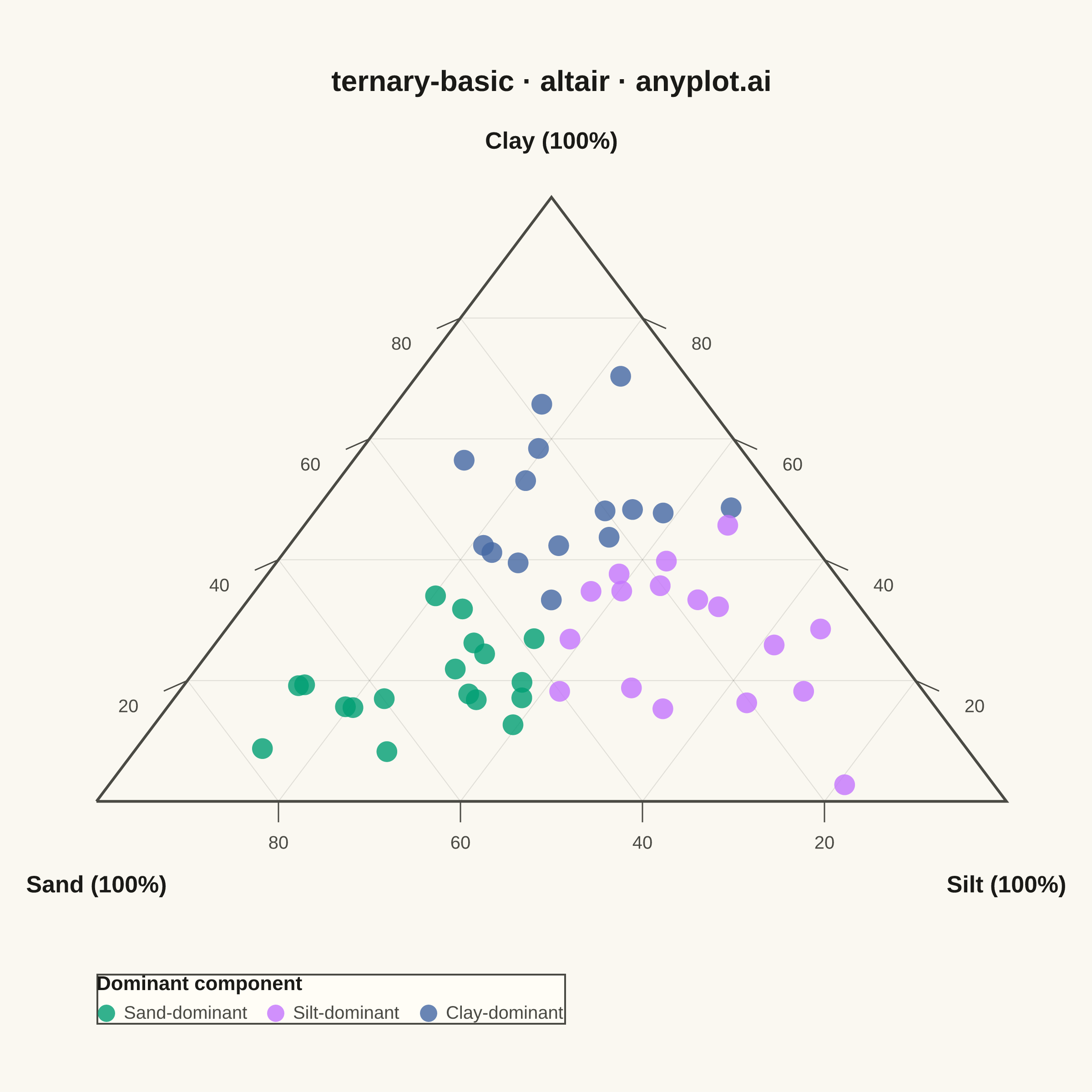
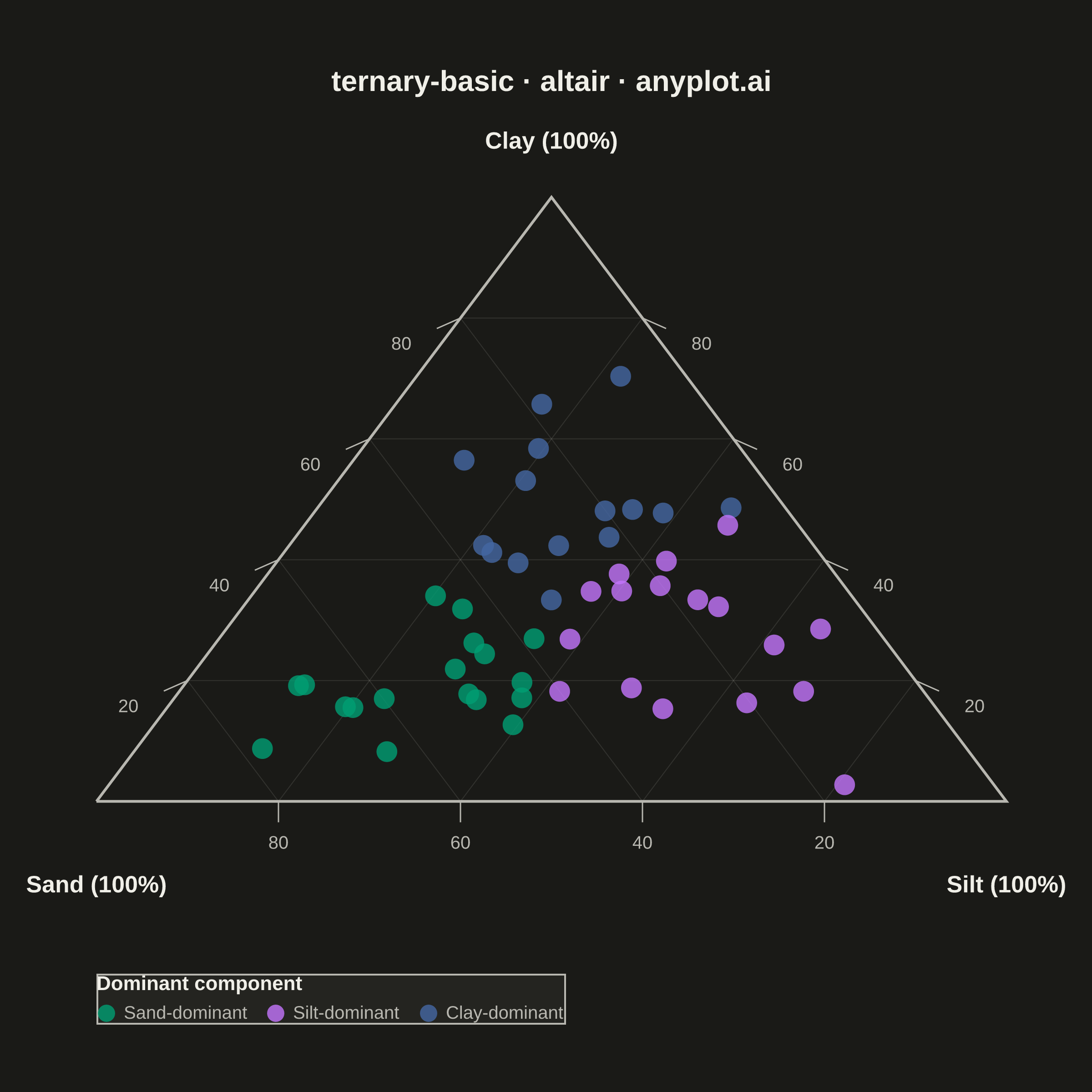
A ternary plot displays three-component compositional data on an equilateral triangle where each vertex represents 100% of one component. Points inside the triangle show compositions that sum to a constant total (usually 100%), with position indicating relative proportions. This visualization is essential for data where three variables are interdependent and constrained to sum to a fixed value.
""" anyplot.ai
ternary-basic: Basic Ternary Plot
Library: altair 6.2.2 | Python 3.13.14
Quality: 90/100 | Updated: 2026-08-04
"""

import os
import sys

import numpy as np
import pandas as pd
from PIL import Image


# Clean sys.path early to avoid importing this file as 'altair' (file naming conflict)
_script_dir = os.path.dirname(os.path.abspath(__file__))
while _script_dir in sys.path:
    sys.path.remove(_script_dir)

import altair as alt


# Theme tokens (Imprint)
THEME = os.getenv("ANYPLOT_THEME", "light")
PAGE_BG = "#FAF8F1" if THEME == "light" else "#1A1A17"
ELEVATED_BG = "#FFFDF6" if THEME == "light" else "#242420"
INK = "#1A1A17" if THEME == "light" else "#F0EFE8"
INK_SOFT = "#4A4A44" if THEME == "light" else "#B8B7B0"
IMPRINT_PALETTE = ["#009E73", "#C475FD", "#4467A3"]  # Imprint positions 1-3

# Data - Soil composition samples (sand, silt, clay)
np.random.seed(42)
n_points = 50

# Generate random compositional data that sums to 100
raw = np.random.dirichlet([2, 2, 2], size=n_points) * 100
sand = raw[:, 0]
silt = raw[:, 1]
clay = raw[:, 2]

# Ternary to Cartesian conversion
# In a standard ternary plot with equilateral triangle:
# - Bottom-left vertex (0,0): 100% Sand
# - Bottom-right vertex (1,0): 100% Silt
# - Top vertex (0.5, sqrt(3)/2): 100% Clay
height = np.sqrt(3) / 2
total = sand + silt + clay
x = silt / total + 0.5 * clay / total
y = clay / total * height

# Classify each sample by its dominant component -- gives the point cloud a
# focal data story (three texture groups radiating from their vertex) instead
# of one undifferentiated color blob.
dominant_idx = np.argmax(np.stack([sand, silt, clay], axis=1), axis=1)
texture = np.array(["Sand-dominant", "Silt-dominant", "Clay-dominant"])[dominant_idx]

df = pd.DataFrame(
    {
        "x": x,
        "y": y,
        "Sand (%)": sand.round(1),
        "Silt (%)": silt.round(1),
        "Clay (%)": clay.round(1),
        "Texture": texture,
    }
)

# Create triangle outline
triangle_vertices = pd.DataFrame({"x": [0, 1, 0.5, 0], "y": [0, 0, height, 0], "order": [0, 1, 2, 3]})

# Create grid lines at 20% intervals
grid_lines = []

for pct in [20, 40, 60, 80]:
    # Lines parallel to bottom edge (constant clay)
    a1, b1, c1 = 100 - pct, 0, pct
    a2, b2, c2 = 0, 100 - pct, pct
    x1 = b1 / 100 + 0.5 * c1 / 100
    y1 = c1 / 100 * height
    x2 = b2 / 100 + 0.5 * c2 / 100
    y2 = c2 / 100 * height
    grid_lines.append({"x": x1, "y": y1, "x2": x2, "y2": y2})

    # Lines parallel to left edge (constant silt)
    a1, b1, c1 = 100 - pct, pct, 0
    a2, b2, c2 = 0, pct, 100 - pct
    x1 = b1 / 100 + 0.5 * c1 / 100
    y1 = c1 / 100 * height
    x2 = b2 / 100 + 0.5 * c2 / 100
    y2 = c2 / 100 * height
    grid_lines.append({"x": x1, "y": y1, "x2": x2, "y2": y2})

    # Lines parallel to right edge (constant sand)
    a1, b1, c1 = pct, 100 - pct, 0
    a2, b2, c2 = pct, 0, 100 - pct
    x1 = b1 / 100 + 0.5 * c1 / 100
    y1 = c1 / 100 * height
    x2 = b2 / 100 + 0.5 * c2 / 100
    y2 = c2 / 100 * height
    grid_lines.append({"x": x1, "y": y1, "x2": x2, "y2": y2})

grid_df = pd.DataFrame(grid_lines)

# Create tick marks along each edge (exclude 0 and 100 to avoid vertex overlap)
tick_data = []
tick_length = 0.03

for pct in [20, 40, 60, 80]:
    # Bottom edge ticks (sand axis) - from left (100%) to right (0%)
    tx = pct / 100
    tick_data.append(
        {"x": tx, "y": 0, "x2": tx, "y2": -tick_length, "label": str(100 - pct), "label_x": tx, "label_y": -0.06}
    )

    # Left edge ticks (clay axis) - from bottom (0%) to top (100%)
    cx = 0.5 * pct / 100
    cy = pct / 100 * height
    dx = -tick_length * np.cos(np.pi / 6)
    dy = -tick_length * np.sin(np.pi / 6)
    tick_data.append(
        {
            "x": cx,
            "y": cy,
            "x2": cx + dx,
            "y2": cy + dy,
            "label": str(pct),
            "label_x": cx + dx * 2.5,
            "label_y": cy + dy * 2.5,
        }
    )

    # Right edge ticks (silt axis) - from bottom (0%) to top (100%)
    sx = 1 - 0.5 * pct / 100
    sy = pct / 100 * height
    dx = tick_length * np.cos(np.pi / 6)
    dy = -tick_length * np.sin(np.pi / 6)
    tick_data.append(
        {
            "x": sx,
            "y": sy,
            "x2": sx + dx,
            "y2": sy + dy,
            "label": str(pct),
            "label_x": sx + dx * 2.5,
            "label_y": sy + dy * 2.5,
        }
    )

tick_df = pd.DataFrame(tick_data)

# Vertex labels
vertex_labels = pd.DataFrame(
    {"x": [0, 1, 0.5], "y": [-0.12, -0.12, height + 0.08], "label": ["Sand (100%)", "Silt (100%)", "Clay (100%)"]}
)

# Triangle outline
triangle = (
    alt.Chart(triangle_vertices)
    .mark_line(strokeWidth=1.5, color=INK_SOFT)
    .encode(x=alt.X("x:Q"), y=alt.Y("y:Q"), order="order:O")
)

# Grid lines
grid = (
    alt.Chart(grid_df)
    .mark_rule(strokeWidth=0.5, opacity=0.15, color=INK_SOFT)
    .encode(x="x:Q", y="y:Q", x2="x2:Q", y2="y2:Q")
)

# Tick marks
ticks = alt.Chart(tick_df).mark_rule(strokeWidth=0.75, color=INK_SOFT).encode(x="x:Q", y="y:Q", x2="x2:Q", y2="y2:Q")

# Tick labels
tick_labels = (
    alt.Chart(tick_df).mark_text(fontSize=10, color=INK_SOFT).encode(x="label_x:Q", y="label_y:Q", text="label:N")
)

# Vertex labels
vertex_text = (
    alt.Chart(vertex_labels)
    .mark_text(fontSize=13, fontWeight="bold", color=INK)
    .encode(x="x:Q", y="y:Q", text="label:N")
)

# Data points - colored by dominant component, Imprint palette positions 1-3
points = (
    alt.Chart(df)
    .mark_point(filled=True, size=130, opacity=0.8)
    .encode(
        x="x:Q",
        y="y:Q",
        color=alt.Color(
            "Texture:N",
            scale=alt.Scale(domain=["Sand-dominant", "Silt-dominant", "Clay-dominant"], range=IMPRINT_PALETTE),
            legend=alt.Legend(
                title="Dominant component",
                orient="bottom",
                direction="horizontal",
                titleColor=INK,
                labelColor=INK_SOFT,
                fillColor=ELEVATED_BG,
                strokeColor=INK_SOFT,
                symbolSize=90,
            ),
        ),
        tooltip=[
            alt.Tooltip("Sand (%):Q", format=".1f"),
            alt.Tooltip("Silt (%):Q", format=".1f"),
            alt.Tooltip("Clay (%):Q", format=".1f"),
            alt.Tooltip("Texture:N"),
        ],
    )
)

# Combine all layers and hide default axes
chart = (
    alt.layer(grid, triangle, ticks, tick_labels, vertex_text, points)
    .properties(
        width=500,
        height=460,
        background=PAGE_BG,
        title=alt.Title(text="ternary-basic · altair · anyplot.ai", fontSize=16, color=INK),
    )
    .configure_axis(grid=False, domain=False, ticks=False, labels=False, title=None)
    .configure_view(strokeWidth=0, fill=PAGE_BG)
)

# Square canvas: the triangle's natural aspect ratio (base 1.0, height sqrt(3)/2
# plus label margins) is close to 1:1, so a square canvas wastes far less
# horizontal space than landscape would.
chart.save(f"plot-{THEME}.png", scale_factor=4.0)

# vl-convert pads the view with title/label extents outside width/height, so the
# saved PNG is larger than (width * scale_factor, height * scale_factor). PAD
# (never crop) up to the exact canonical target.
TW, TH = 2400, 2400
_img = Image.open(f"plot-{THEME}.png").convert("RGB")
_w, _h = _img.size
if _w > TW or _h > TH:
    raise SystemExit(
        f"altair vl-convert produced {_w}x{_h}, exceeds target {TW}x{TH}. "
        f"Shrink chart .properties(width=, height=) values and re-render."
    )
if _w < TW or _h < TH:
    _canvas = Image.new("RGB", (TW, TH), PAGE_BG)
    _canvas.paste(_img, ((TW - _w) // 2, (TH - _h) // 2))
    _canvas.save(f"plot-{THEME}.png")

chart.save(f"plot-{THEME}.html")
Runnable source as JSON, for any HTTP client: https://api.anyplot.ai/specs/ternary-basic/altair/code. Any spec id and library id listed in llms-full.txt fit the same URL shape; every URL below is complete and callable.
{
  "spec_id": "ternary-basic",
  "language": "python",
  "library": "altair",
  "page": "https://anyplot.ai/ternary-basic/python/altair",
  "hub": "https://anyplot.ai/ternary-basic",
  "code_json": "https://api.anyplot.ai/specs/ternary-basic/altair/code",
  "spec_json": "https://api.anyplot.ai/specs/ternary-basic",
  "render_light_png": "https://storage.googleapis.com/anyplot-images/plots/ternary-basic/python/altair/plot-light.png",
  "render_dark_png": "https://storage.googleapis.com/anyplot-images/plots/ternary-basic/python/altair/plot-dark.png",
  "interactive_light_html": "https://storage.googleapis.com/anyplot-images/plots/ternary-basic/python/altair/plot-light.html",
  "interactive_dark_html": "https://storage.googleapis.com/anyplot-images/plots/ternary-basic/python/altair/plot-dark.html",
  "quality_score": 90.0,
  "license": "MIT",
  "guide": "https://anyplot.ai/llms.txt"
}
Part of Basic Ternary Plot on anyplot.ai.