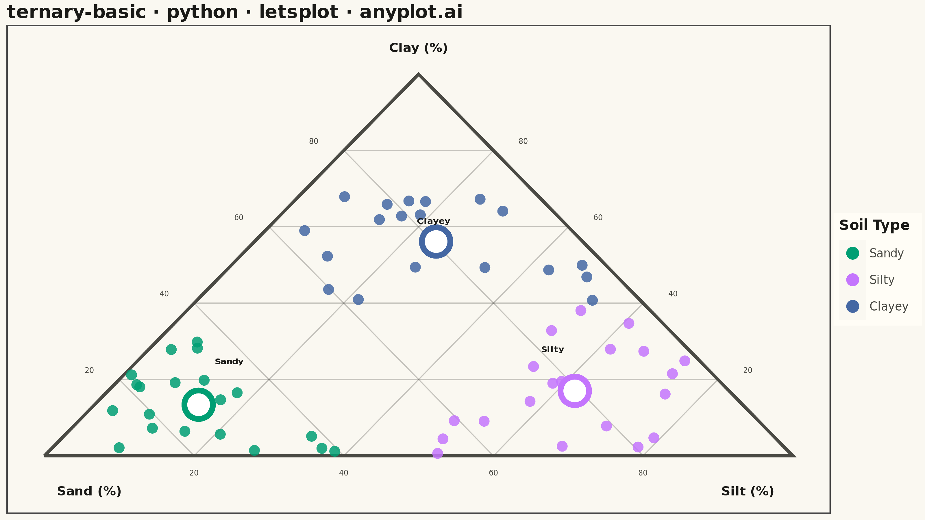
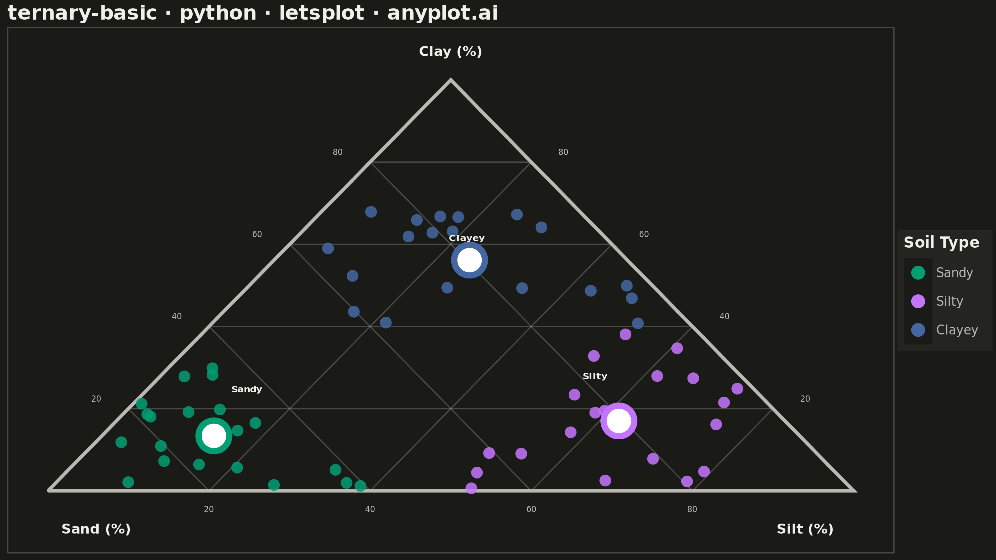
A ternary plot displays three-component compositional data on an equilateral triangle where each vertex represents 100% of one component. Points inside the triangle show compositions that sum to a constant total (usually 100%), with position indicating relative proportions. This visualization is essential for data where three variables are interdependent and constrained to sum to a fixed value.
""" anyplot.ai
ternary-basic: Basic Ternary Plot
Library: letsplot 4.11.0 | Python 3.13.14
Quality: 92/100 | Updated: 2026-08-04
"""

import os

import numpy as np
import pandas as pd
from lets_plot import (
    LetsPlot,
    aes,
    element_blank,
    element_rect,
    element_text,
    geom_point,
    geom_polygon,
    geom_segment,
    geom_text,
    ggplot,
    ggsave,
    ggsize,
    labs,
    layer_tooltips,
    scale_color_manual,
    theme,
)


LetsPlot.setup_html()

# Theme tokens
THEME = os.getenv("ANYPLOT_THEME", "light")
PAGE_BG = "#FAF8F1" if THEME == "light" else "#1A1A17"
ELEVATED_BG = "#FFFDF6" if THEME == "light" else "#242420"
INK = "#1A1A17" if THEME == "light" else "#F0EFE8"
INK_SOFT = "#4A4A44" if THEME == "light" else "#B8B7B0"

# Imprint palette (categorical, positions 1-3)
IMPRINT = ["#009E73", "#C475FD", "#4467A3"]

# Data: Soil composition samples (Sand, Silt, Clay)
np.random.seed(42)

# Generate realistic soil composition data in different soil type regions
samples = []
soil_types = []

# Sandy soils (high sand)
for _ in range(20):
    sand = np.random.uniform(60, 90)
    remaining = 100 - sand
    silt = np.random.uniform(0, remaining)
    clay = remaining - silt
    samples.append((sand, silt, clay))
    soil_types.append("Sandy")

# Silty soils (high silt)
for _ in range(20):
    silt = np.random.uniform(50, 80)
    remaining = 100 - silt
    sand = np.random.uniform(0, remaining)
    clay = remaining - sand
    samples.append((sand, silt, clay))
    soil_types.append("Silty")

# Clay soils (high clay)
for _ in range(20):
    clay = np.random.uniform(40, 70)
    remaining = 100 - clay
    sand = np.random.uniform(0, remaining)
    silt = remaining - sand
    samples.append((sand, silt, clay))
    soil_types.append("Clayey")

# Convert ternary to Cartesian coordinates
# Formula: x = 0.5 * (2*b + c) / (a+b+c), y = sqrt(3)/2 * c / (a+b+c)
# where a=Sand (bottom-left), b=Silt (bottom-right), c=Clay (top)
sqrt3_2 = np.sqrt(3) / 2
x_coords = []
y_coords = []
for sand, silt, clay in samples:
    total = sand + silt + clay
    silt_norm = silt / total
    clay_norm = clay / total
    x_coords.append(0.5 * (2 * silt_norm + clay_norm))
    y_coords.append(sqrt3_2 * clay_norm)

df = pd.DataFrame(
    {
        "x": x_coords,
        "y": y_coords,
        "soil_type": soil_types,
        "sand": [round(s, 1) for s, _, _ in samples],
        "silt": [round(s, 1) for _, s, _ in samples],
        "clay": [round(c, 1) for _, _, c in samples],
    }
)

# Triangle vertices (Sand at bottom-left, Silt at bottom-right, Clay at top)
vertices = pd.DataFrame({"x": [0, 1, 0.5, 0], "y": [0, 0, sqrt3_2, 0]})

# Grid lines at 20% intervals
grid_segments = []
for pct in [0.2, 0.4, 0.6, 0.8]:
    # Lines parallel to Sand-Silt edge (constant Clay)
    x1 = 0.5 * (0 + pct)
    y1 = sqrt3_2 * pct
    x2 = 0.5 * (2 * (1 - pct) + pct)
    y2 = sqrt3_2 * pct
    grid_segments.append({"x": x1, "y": y1, "xend": x2, "yend": y2})

    # Lines parallel to Sand-Clay edge (constant Silt)
    x1 = 0.5 * (2 * pct + 0)
    y1 = 0
    x2 = 0.5 * (2 * pct + (1 - pct))
    y2 = sqrt3_2 * (1 - pct)
    grid_segments.append({"x": x1, "y": y1, "xend": x2, "yend": y2})

    # Lines parallel to Silt-Clay edge (constant Sand)
    x1 = 0.5 * (2 * (1 - pct) + 0)
    y1 = 0
    x2 = 0.5 * (0 + (1 - pct))
    y2 = sqrt3_2 * (1 - pct)
    grid_segments.append({"x": x1, "y": y1, "xend": x2, "yend": y2})

grid_df = pd.DataFrame(grid_segments)

# Vertex labels with offset for readability
label_offset = 0.06
labels_df = pd.DataFrame(
    {
        "x": [0 + label_offset, 1 - label_offset, 0.5],
        "y": [-label_offset - 0.02, -label_offset - 0.02, sqrt3_2 + label_offset],
        "label": ["Sand (%)", "Silt (%)", "Clay (%)"],
    }
)

# Tick labels along edges (at 20%, 40%, 60%, 80%)
tick_labels = []
for pct in [20, 40, 60, 80]:
    frac = pct / 100
    # Along left edge
    x = 0.5 * frac
    y = sqrt3_2 * frac
    tick_labels.append({"x": x - 0.04, "y": y + 0.02, "label": str(pct)})

    # Along right edge
    x = 0.5 * (2 * (1 - frac) + frac)
    y = sqrt3_2 * frac
    tick_labels.append({"x": x + 0.04, "y": y + 0.02, "label": str(pct)})

    # Along bottom edge
    x = 0.5 * (2 * frac)
    y = 0
    tick_labels.append({"x": x, "y": y - 0.04, "label": str(pct)})

tick_df = pd.DataFrame(tick_labels)

# Cluster centroids nudged toward the triangle center, for a storytelling
# callout per region beyond plain color-coded scatter.
tri_center_x, tri_center_y = 0.5, sqrt3_2 / 3
centroid_df = df.groupby("soil_type", as_index=False)[["x", "y"]].mean()
centroid_df["label_x"] = centroid_df["x"] + 0.14 * (tri_center_x - centroid_df["x"])
centroid_df["label_y"] = centroid_df["y"] + 0.14 * (tri_center_y - centroid_df["y"]) + 0.075

# Distinctive letsplot feature: interactive per-point tooltips carrying the
# exact composition (not just position) — surfaced in the exported HTML.
point_tooltips = (
    layer_tooltips().line("Soil type|@soil_type").line("Sand (%)|@sand").line("Silt (%)|@silt").line("Clay (%)|@clay")
)

# Plot
plot = (
    ggplot()
    # Triangle outline
    + geom_polygon(data=vertices, mapping=aes(x="x", y="y"), fill=PAGE_BG, color=INK_SOFT, size=1.2, alpha=1)
    # Grid lines
    + geom_segment(
        data=grid_df, mapping=aes(x="x", y="y", xend="xend", yend="yend"), color=INK_SOFT, size=0.4, alpha=0.3
    )
    # Data points
    + geom_point(data=df, mapping=aes(x="x", y="y", color="soil_type"), size=4.2, alpha=0.85, tooltips=point_tooltips)
    # Cluster centroid markers (ring) + labels, calling out each soil region
    + geom_point(
        data=centroid_df,
        mapping=aes(x="x", y="y", color="soil_type"),
        size=9,
        shape=21,
        fill="white",
        stroke=2.2,
        show_legend=False,
    )
    + geom_text(
        data=centroid_df, mapping=aes(x="label_x", y="label_y", label="soil_type"), size=3.8, fontface="bold", color=INK
    )
    # Vertex labels
    + geom_text(data=labels_df, mapping=aes(x="x", y="y", label="label"), size=5.5, fontface="bold", color=INK)
    # Tick labels
    + geom_text(data=tick_df, mapping=aes(x="x", y="y", label="label"), size=3.2, color=INK_SOFT)
    # Color scale using Imprint palette
    + scale_color_manual(values=IMPRINT)
    # Labels and title
    + labs(title="ternary-basic · python · letsplot · anyplot.ai", color="Soil Type")
    # Theme
    + theme(
        plot_background=element_rect(fill=PAGE_BG, color=PAGE_BG),
        panel_background=element_rect(fill=PAGE_BG),
        plot_title=element_text(size=16, face="bold", color=INK),
        legend_background=element_rect(fill=ELEVATED_BG, color=INK_SOFT),
        legend_title=element_text(size=12, color=INK, face="bold"),
        legend_text=element_text(size=10, color=INK_SOFT),
        axis_title=element_blank(),
        axis_text=element_blank(),
        axis_ticks=element_blank(),
        axis_line=element_blank(),
        panel_grid=element_blank(),
        legend_position="right",
    )
    + ggsize(800, 450)
)

# Save as PNG (scale 4x to get 3200 x 1800 px) and HTML
ggsave(plot, f"plot-{THEME}.png", path=".", scale=4)
ggsave(plot, f"plot-{THEME}.html", path=".")
Runnable source as JSON, for any HTTP client: https://api.anyplot.ai/specs/ternary-basic/letsplot/code. Any spec id and library id listed in llms-full.txt fit the same URL shape; every URL below is complete and callable.
{
  "spec_id": "ternary-basic",
  "language": "python",
  "library": "letsplot",
  "page": "https://anyplot.ai/ternary-basic/python/letsplot",
  "hub": "https://anyplot.ai/ternary-basic",
  "code_json": "https://api.anyplot.ai/specs/ternary-basic/letsplot/code",
  "spec_json": "https://api.anyplot.ai/specs/ternary-basic",
  "render_light_png": "https://storage.googleapis.com/anyplot-images/plots/ternary-basic/python/letsplot/plot-light.png",
  "render_dark_png": "https://storage.googleapis.com/anyplot-images/plots/ternary-basic/python/letsplot/plot-dark.png",
  "interactive_light_html": "https://storage.googleapis.com/anyplot-images/plots/ternary-basic/python/letsplot/plot-light.html",
  "interactive_dark_html": "https://storage.googleapis.com/anyplot-images/plots/ternary-basic/python/letsplot/plot-dark.html",
  "quality_score": 92.0,
  "license": "MIT",
  "guide": "https://anyplot.ai/llms.txt"
}
Part of Basic Ternary Plot on anyplot.ai.