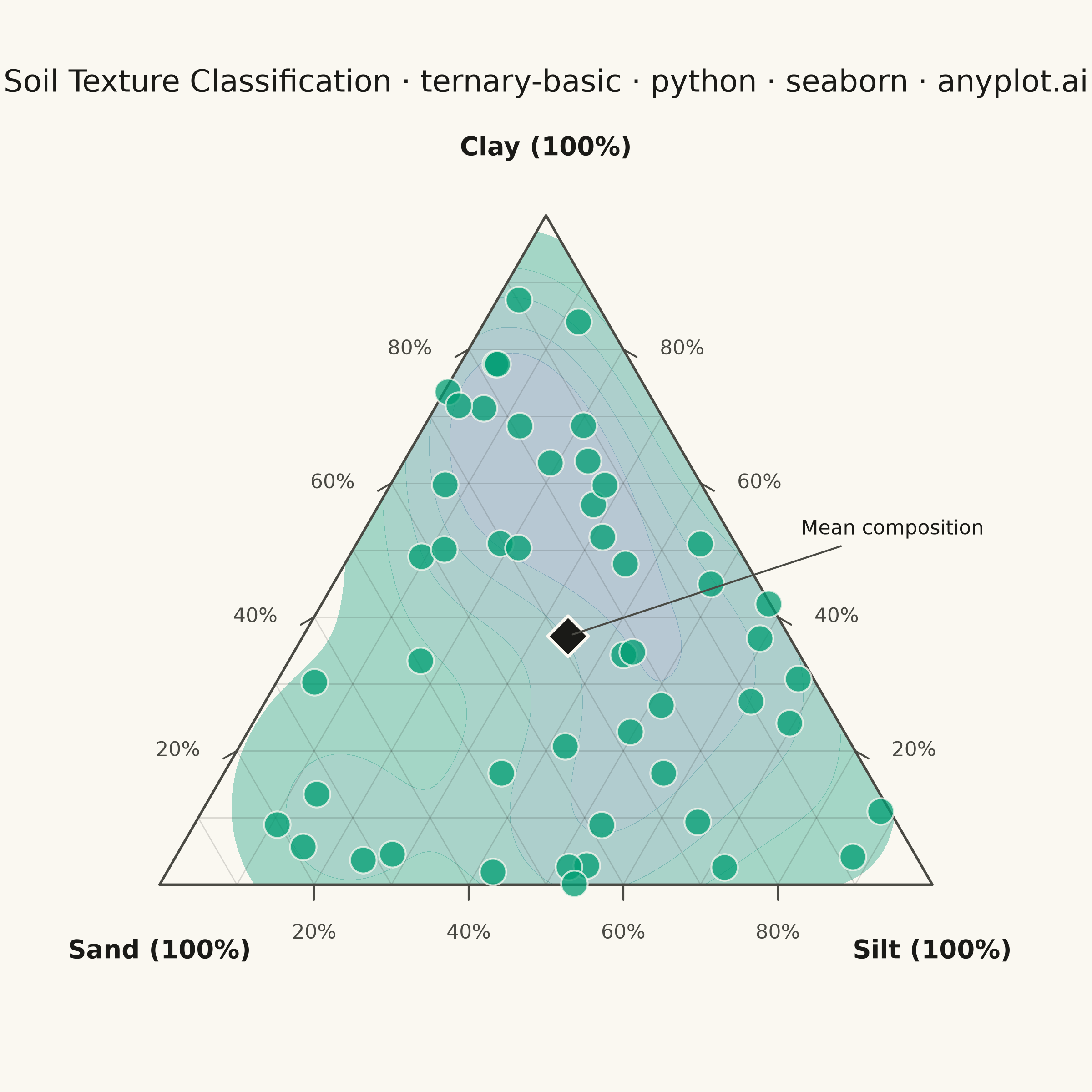
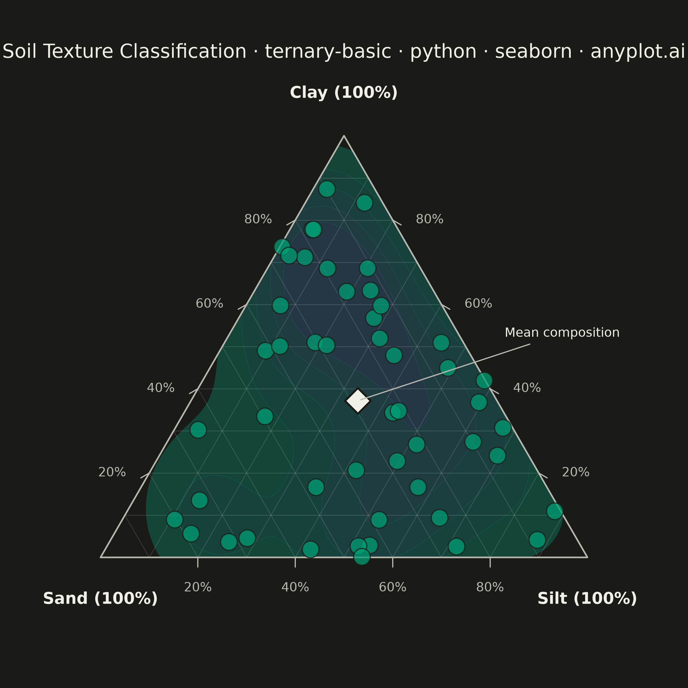
A ternary plot displays three-component compositional data on an equilateral triangle where each vertex represents 100% of one component. Points inside the triangle show compositions that sum to a constant total (usually 100%), with position indicating relative proportions. This visualization is essential for data where three variables are interdependent and constrained to sum to a fixed value.
""" anyplot.ai
ternary-basic: Basic Ternary Plot
Library: seaborn 0.13.2 | Python 3.13.14
Quality: 85/100 | Updated: 2026-08-04
"""

import os
import sys


# Remove script directory from sys.path to avoid local matplotlib.py shadow
script_dir = os.path.dirname(os.path.abspath(__file__))
sys.path = [p for p in sys.path if os.path.abspath(p) != script_dir]

import matplotlib.pyplot as plt
import numpy as np
import pandas as pd
import seaborn as sns
from matplotlib.colors import LinearSegmentedColormap
from matplotlib.patches import Polygon


# Theme tokens (see prompts/default-style-guide.md)
THEME = os.getenv("ANYPLOT_THEME", "light")
PAGE_BG = "#FAF8F1" if THEME == "light" else "#1A1A17"
INK = "#1A1A17" if THEME == "light" else "#F0EFE8"
INK_SOFT = "#4A4A44" if THEME == "light" else "#B8B7B0"
BRAND = "#009E73"  # Okabe-Ito position 1
imprint_seq = LinearSegmentedColormap.from_list("imprint_seq", ["#009E73", "#4467A3"])

# Set seaborn/matplotlib theme
sns.set_theme(
    style="ticks",
    rc={
        "figure.facecolor": PAGE_BG,
        "axes.facecolor": PAGE_BG,
        "axes.edgecolor": INK_SOFT,
        "axes.labelcolor": INK,
        "text.color": INK,
        "xtick.color": INK_SOFT,
        "ytick.color": INK_SOFT,
        "grid.color": INK,
        "grid.alpha": 0.15,
    },
)

# Data - Soil texture samples (Sand, Silt, Clay), USDA-style ternary domain
# alpha=1 draws uniformly over the simplex, giving realistic coverage all the
# way to near-pure single-component corners (unlike a peaked Dirichlet).
np.random.seed(42)
n_points = 50
raw = np.random.dirichlet(alpha=[1.0, 1.0, 1.0], size=n_points) * 100
df = pd.DataFrame({"Sand": raw[:, 0], "Silt": raw[:, 1], "Clay": raw[:, 2]})

# Ternary coordinates transformation (vectorized)
# Convert (a, b, c) to Cartesian (x, y) where a + b + c = 100
# Triangle vertices: Bottom-left (0,0)=Sand, Bottom-right (1,0)=Silt, Top (0.5, sqrt(3)/2)=Clay
sqrt3_2 = np.sqrt(3) / 2
sand_norm = df["Sand"].values / 100
silt_norm = df["Silt"].values / 100
clay_norm = df["Clay"].values / 100
x = 0.5 * (2 * silt_norm + clay_norm)
y = sqrt3_2 * clay_norm
scatter_df = pd.DataFrame({"x": x, "y": y})

# Create plot — canonical square canvas: figsize(6,6) x dpi=400 -> 2400x2400 px
fig, ax = plt.subplots(figsize=(6, 6), dpi=400, facecolor=PAGE_BG)

# Triangle outline (used both for drawing and as a density clip mask)
triangle = np.array([[0, 0], [1, 0], [0.5, sqrt3_2], [0, 0]])

# Density backdrop — genuine seaborn statistical estimator (KDE), clipped to
# the simplex, to give the point cloud a visual hierarchy instead of a flat
# scatter (addresses DE-03 storytelling + LM-02 distinctive-feature usage).
existing_collections = set(ax.collections)
sns.kdeplot(
    x=scatter_df["x"],
    y=scatter_df["y"],
    ax=ax,
    fill=True,
    cmap=imprint_seq,
    alpha=0.35,
    levels=6,
    thresh=0.15,
    zorder=1,
)
clip_patch = Polygon(triangle[:-1], transform=ax.transData)
for collection in ax.collections:
    if collection not in existing_collections:
        collection.set_clip_path(clip_patch)

# Draw triangle outline
ax.plot(triangle[:, 0], triangle[:, 1], color=INK_SOFT, linewidth=1, zorder=5)

# Draw grid lines at 10% intervals
grid_lw = 0.5

for level in [0.1, 0.2, 0.3, 0.4, 0.5, 0.6, 0.7, 0.8, 0.9]:
    # Lines parallel to bottom (constant Clay)
    x1, y1 = 0.5 * level, sqrt3_2 * level
    x2, y2 = 1 - 0.5 * level, sqrt3_2 * level
    ax.plot([x1, x2], [y1, y2], color=INK, alpha=0.15, linewidth=grid_lw, zorder=2)

    # Lines parallel to left edge (constant Silt)
    x1, y1 = level, 0
    x2, y2 = 0.5 + 0.5 * level, sqrt3_2 * (1 - level)
    ax.plot([x1, x2], [y1, y2], color=INK, alpha=0.15, linewidth=grid_lw, zorder=2)

    # Lines parallel to right edge (constant Sand)
    x1, y1 = 0.5 * (1 - level), sqrt3_2 * (1 - level)
    x2, y2 = 1 - level, 0
    ax.plot([x1, x2], [y1, y2], color=INK, alpha=0.15, linewidth=grid_lw, zorder=2)

# Add tick marks along edges (at 20% intervals)
tick_length = 0.02

for level in [0.2, 0.4, 0.6, 0.8]:
    # Bottom edge ticks (Silt percentage increasing left to right)
    ax.plot([level, level], [-tick_length, 0], color=INK_SOFT, linewidth=0.75, zorder=5)
    ax.text(level, -0.05, f"{int(level * 100)}%", ha="center", va="top", fontsize=8, color=INK_SOFT)

    # Left edge ticks (Clay percentage)
    x_tick = 0.5 * level
    y_tick = sqrt3_2 * level
    dx, dy = -tick_length * np.cos(np.pi / 6), -tick_length * np.sin(np.pi / 6)
    ax.plot([x_tick, x_tick + dx], [y_tick, y_tick + dy], color=INK_SOFT, linewidth=0.75, zorder=5)
    ax.text(
        x_tick + dx - 0.03,
        y_tick + dy + 0.01,
        f"{int(level * 100)}%",
        ha="right",
        va="center",
        fontsize=8,
        color=INK_SOFT,
    )

    # Right edge ticks (Clay percentage from right side)
    x_tick = 1 - 0.5 * level
    y_tick = sqrt3_2 * level
    dx, dy = tick_length * np.cos(np.pi / 6), -tick_length * np.sin(np.pi / 6)
    ax.plot([x_tick, x_tick + dx], [y_tick, y_tick + dy], color=INK_SOFT, linewidth=0.75, zorder=5)
    ax.text(
        x_tick + dx + 0.03,
        y_tick + dy + 0.01,
        f"{int(level * 100)}%",
        ha="left",
        va="center",
        fontsize=8,
        color=INK_SOFT,
    )

# Data points — routed through seaborn's own plotting API (not raw ax.scatter)
sns.scatterplot(
    data=scatter_df,
    x="x",
    y="y",
    ax=ax,
    color=BRAND,
    s=110,
    alpha=0.75,
    edgecolor=PAGE_BG,
    linewidth=0.75,
    zorder=10,
    legend=False,
)

# Centroid marker — highlights the dataset's average composition for a
# guided reading instead of a flat, unannotated point cloud.
centroid_x, centroid_y = scatter_df["x"].mean(), scatter_df["y"].mean()
ax.scatter([centroid_x], [centroid_y], marker="D", s=130, facecolor=INK, edgecolor=PAGE_BG, linewidth=1.2, zorder=11)
ax.annotate(
    "Mean composition",
    xy=(centroid_x, centroid_y),
    xytext=(0.83, 0.46),
    fontsize=8,
    color=INK,
    ha="left",
    va="center",
    zorder=12,
    arrowprops={"arrowstyle": "-", "color": INK_SOFT, "linewidth": 0.75},
)

# Vertex labels
label_offset = 0.07
ax.text(0, -label_offset, "Sand (100%)", ha="center", va="top", fontsize=10, fontweight="bold", color=INK)
ax.text(1, -label_offset, "Silt (100%)", ha="center", va="top", fontsize=10, fontweight="bold", color=INK)
ax.text(0.5, sqrt3_2 + label_offset, "Clay (100%)", ha="center", va="bottom", fontsize=10, fontweight="bold", color=INK)

# Title — mandated format: {Descriptive Title} · {spec-id} · {language} · {library} · anyplot.ai
ax.set_title(
    "Soil Texture Classification · ternary-basic · python · seaborn · anyplot.ai",
    fontsize=12,
    pad=8,
    color=INK,
    fontweight="medium",
)

# Clean up axes — tighter top margin than the previous revision to balance
# the title-to-apex gap against the base-to-bottom-edge gap (VQ-05).
ax.set_xlim(-0.15, 1.15)
ax.set_ylim(-0.18, 1.0)
ax.set_aspect("equal")
ax.axis("off")

fig.subplots_adjust(left=0.04, right=0.96, top=0.90, bottom=0.06)
plt.savefig(f"plot-{THEME}.png", dpi=400, facecolor=PAGE_BG)  # bbox_inches MUST stay default (None) — see canvas rule
Runnable source as JSON, for any HTTP client: https://api.anyplot.ai/specs/ternary-basic/seaborn/code. Any spec id and library id listed in llms-full.txt fit the same URL shape; every URL below is complete and callable.
{
  "spec_id": "ternary-basic",
  "language": "python",
  "library": "seaborn",
  "page": "https://anyplot.ai/ternary-basic/python/seaborn",
  "hub": "https://anyplot.ai/ternary-basic",
  "code_json": "https://api.anyplot.ai/specs/ternary-basic/seaborn/code",
  "spec_json": "https://api.anyplot.ai/specs/ternary-basic",
  "render_light_png": "https://storage.googleapis.com/anyplot-images/plots/ternary-basic/python/seaborn/plot-light.png",
  "render_dark_png": "https://storage.googleapis.com/anyplot-images/plots/ternary-basic/python/seaborn/plot-dark.png",
  "quality_score": 85.0,
  "license": "MIT",
  "guide": "https://anyplot.ai/llms.txt"
}
Part of Basic Ternary Plot on anyplot.ai.