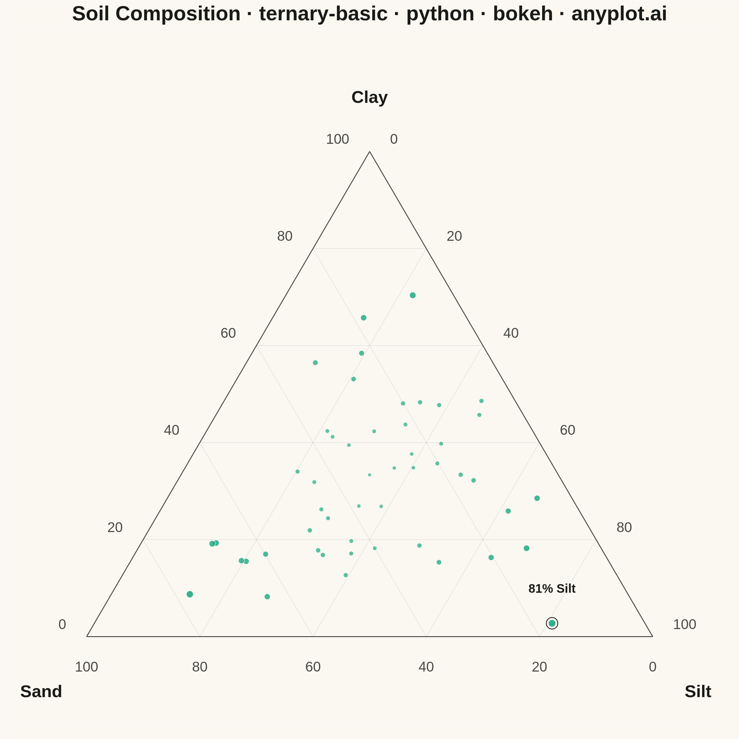
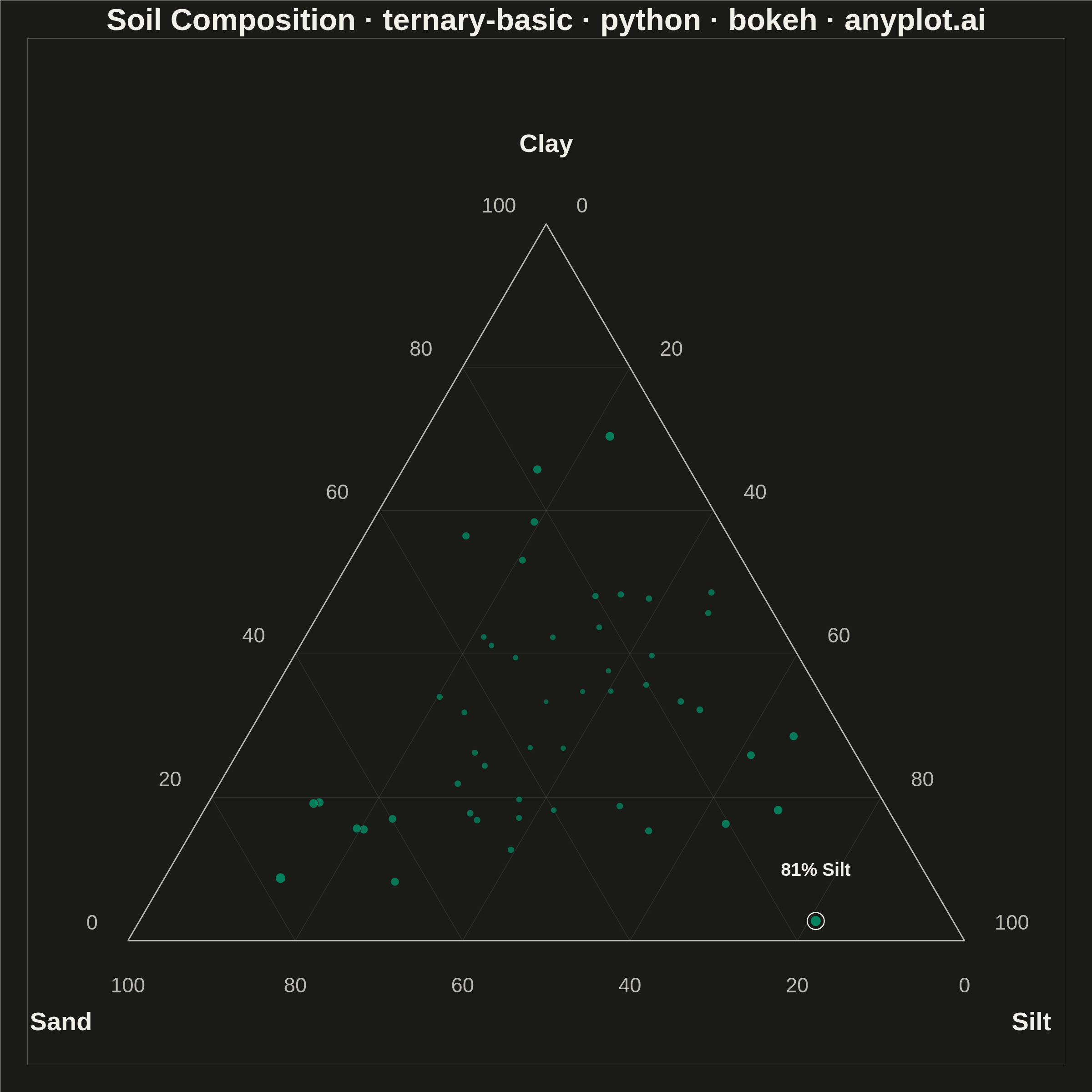
A ternary plot displays three-component compositional data on an equilateral triangle where each vertex represents 100% of one component. Points inside the triangle show compositions that sum to a constant total (usually 100%), with position indicating relative proportions. This visualization is essential for data where three variables are interdependent and constrained to sum to a fixed value.
""" anyplot.ai
ternary-basic: Basic Ternary Plot
Library: bokeh 3.9.2 | Python 3.13.14
Quality: 92/100 | Created: 2026-08-04
"""

import os
import time
from pathlib import Path

import numpy as np
from bokeh.io import output_file, save
from bokeh.models import ColumnDataSource, HoverTool, Label
from bokeh.plotting import figure
from selenium import webdriver
from selenium.webdriver.chrome.options import Options


THEME = os.getenv("ANYPLOT_THEME", "light")
PAGE_BG = "#FAF8F1" if THEME == "light" else "#1A1A17"
INK = "#1A1A17" if THEME == "light" else "#F0EFE8"
INK_SOFT = "#4A4A44" if THEME == "light" else "#B8B7B0"
BRAND = "#009E73"  # Imprint palette position 1

# Data - Soil composition samples (Sand, Silt, Clay)
np.random.seed(42)
n_points = 50

# Generate random compositions that sum to 100%
raw = np.random.dirichlet(alpha=[2, 2, 2], size=n_points) * 100
sand = raw[:, 0]
silt = raw[:, 1]
clay = raw[:, 2]

# Compositional "purity" (distance from the balanced 1/3-1/3-1/3 centroid) —
# drives the size/opacity emphasis below so near-pure samples pop forward
# and balanced (loam-like) samples recede, surfacing the clustering pattern
# instead of a flat, uniform scatter.
dominance = raw.max(axis=1) / 100
purity = np.clip((dominance - 1 / 3) / (1 - 1 / 3), 0, 1)
marker_size = 12 + purity * 16
marker_alpha = 0.55 + purity * 0.35

# Most extreme sample — the single highest-purity point becomes the plot's
# explicit focal callout, giving viewers a concrete entry point beyond the
# implicit size/alpha gradient.
idx_extreme = int(np.argmax(purity))
extreme_component = ["Sand", "Silt", "Clay"][int(np.argmax(raw[idx_extreme]))]
extreme_pct = raw[idx_extreme].max()


# Convert ternary coordinates to Cartesian (equilateral triangle)
def ternary_to_cartesian(a, b, c):
    """Convert ternary coordinates (a, b, c) to Cartesian (x, y).
    Triangle vertices: bottom-left (1,0,0), bottom-right (0,1,0), top (0,0,1)
    """
    total = a + b + c
    b_norm = b / total
    c_norm = c / total
    x = 0.5 * (2 * b_norm + c_norm)
    y = (np.sqrt(3) / 2) * c_norm
    return x, y


# Convert data points
x_data, y_data = ternary_to_cartesian(sand, silt, clay)

# Triangle vertices (in Cartesian coordinates)
tri_x = [0, 1, 0.5, 0]
tri_y = [0, 0, np.sqrt(3) / 2, 0]

# Create figure. Square canvas: a ternary plot has no preferred horizontal
# axis. Equal-span ranges below (x: -0.12..1.12, y: -0.15..1.09, both span
# 1.24) paired with symmetric min_border on a square figure keep the pixel
# scale uniform in x and y, so the triangle renders truly equilateral.
# HoverTool works as an active inspector even with toolbar_location=None (it
# only shows a toolbar *button*, not the hover behavior), so the static PNG
# render is unaffected while the HTML artifact gains sand/silt/clay tooltips.
hover = HoverTool(tooltips=[("Sand", "@sand{0.0}%"), ("Silt", "@silt{0.0}%"), ("Clay", "@clay{0.0}%")])

p = figure(
    width=2400,
    height=2400,
    title="Soil Composition · ternary-basic · python · bokeh · anyplot.ai",
    x_range=(-0.12, 1.12),
    y_range=(-0.15, 1.09),
    tools=[hover],
    toolbar_location=None,  # IMPORTANT: default toolbar adds ~30-50px, shrinking the saved PNG
    min_border_left=60,
    min_border_right=60,
    min_border_top=60,
    min_border_bottom=60,
)

# Theme styling
p.background_fill_color = PAGE_BG
p.border_fill_color = PAGE_BG
p.outline_line_color = None

# Remove default axes
p.xaxis.visible = False
p.yaxis.visible = False
p.xgrid.visible = False
p.ygrid.visible = False

# Draw triangle outline
p.line(tri_x, tri_y, line_width=3, color=INK_SOFT)

# Draw grid lines at 20% intervals
grid_color = INK_SOFT
grid_alpha = 0.15
grid_width = 1.5

for pct in [20, 40, 60, 80]:
    frac = pct / 100

    # Lines parallel to each side
    a1, b1, c1 = frac, 1 - frac, 0
    a2, b2, c2 = frac, 0, 1 - frac
    x1, y1 = ternary_to_cartesian(a1, b1, c1)
    x2, y2 = ternary_to_cartesian(a2, b2, c2)
    p.line([x1, x2], [y1, y2], line_width=grid_width, color=grid_color, alpha=grid_alpha)

    a1, b1, c1 = 1 - frac, frac, 0
    a2, b2, c2 = 0, frac, 1 - frac
    x1, y1 = ternary_to_cartesian(a1, b1, c1)
    x2, y2 = ternary_to_cartesian(a2, b2, c2)
    p.line([x1, x2], [y1, y2], line_width=grid_width, color=grid_color, alpha=grid_alpha)

    a1, b1, c1 = 1 - frac, 0, frac
    a2, b2, c2 = 0, 1 - frac, frac
    x1, y1 = ternary_to_cartesian(a1, b1, c1)
    x2, y2 = ternary_to_cartesian(a2, b2, c2)
    p.line([x1, x2], [y1, y2], line_width=grid_width, color=grid_color, alpha=grid_alpha)

# Add tick labels along each edge
tick_font_size = "34pt"
tick_offset = 0.045

for pct in [0, 20, 40, 60, 80, 100]:
    frac = pct / 100

    x_tick, y_tick = ternary_to_cartesian(1 - frac, frac, 0)
    label = Label(
        x=x_tick,
        y=y_tick - tick_offset,
        text=f"{int(100 - pct)}",
        text_font_size=tick_font_size,
        text_color=INK_SOFT,
        text_align="center",
        text_baseline="top",
    )
    p.add_layout(label)

    x_tick, y_tick = ternary_to_cartesian(0, 1 - frac, frac)
    label = Label(
        x=x_tick + tick_offset * 0.8,
        y=y_tick + tick_offset * 0.5,
        text=f"{int(100 - pct)}",
        text_font_size=tick_font_size,
        text_color=INK_SOFT,
        text_align="left",
        text_baseline="middle",
    )
    p.add_layout(label)

    x_tick, y_tick = ternary_to_cartesian(frac, 0, 1 - frac)
    label = Label(
        x=x_tick - tick_offset * 0.8,
        y=y_tick + tick_offset * 0.5,
        text=f"{int(100 - pct)}",
        text_font_size=tick_font_size,
        text_color=INK_SOFT,
        text_align="right",
        text_baseline="middle",
    )
    p.add_layout(label)

# Add vertex labels
label_font_size = "42pt"
label_offset = 0.08

sand_label = Label(
    x=0 - label_offset,
    y=0 - label_offset,
    text="Sand",
    text_font_size=label_font_size,
    text_font_style="bold",
    text_color=INK,
    text_align="center",
    text_baseline="top",
)
p.add_layout(sand_label)

silt_label = Label(
    x=1 + label_offset,
    y=0 - label_offset,
    text="Silt",
    text_font_size=label_font_size,
    text_font_style="bold",
    text_color=INK,
    text_align="center",
    text_baseline="top",
)
p.add_layout(silt_label)

clay_label = Label(
    x=0.5,
    y=np.sqrt(3) / 2 + label_offset,
    text="Clay",
    text_font_size=label_font_size,
    text_font_style="bold",
    text_color=INK,
    text_align="center",
    text_baseline="bottom",
)
p.add_layout(clay_label)

# Plot data points — size and opacity scale with compositional purity so
# near-pure (single-component-dominant) samples read as prominent, distinct
# markers while balanced/loam-like samples recede into the cluster.
source = ColumnDataSource(
    data={
        "x": x_data,
        "y": y_data,
        "sand": sand,
        "silt": silt,
        "clay": clay,
        "size": marker_size,
        "alpha": marker_alpha,
    }
)

p.scatter(x="x", y="y", source=source, size="size", color=BRAND, fill_alpha="alpha", line_color=PAGE_BG, line_width=1.5)

# Ring the single most extreme (highest-purity) sample and annotate it —
# an explicit focal callout so the viewer has a concrete entry point into
# the composition space, not just the implicit size/alpha gradient.
p.scatter(
    x=[x_data[idx_extreme]],
    y=[y_data[idx_extreme]],
    size=marker_size[idx_extreme] + 14,
    fill_color=None,
    line_color=INK,
    line_width=2.5,
)
extreme_label = Label(
    x=x_data[idx_extreme],
    y=y_data[idx_extreme] + 0.05,
    text=f"{extreme_pct:.0f}% {extreme_component}",
    text_font_size="30pt",
    text_font_style="bold",
    text_color=INK,
    text_align="center",
    text_baseline="bottom",
)
p.add_layout(extreme_label)

# Style title
p.title.text_font_size = "50pt"
p.title.text_color = INK
p.title.align = "center"

# Save HTML
output_file(f"plot-{THEME}.html")
save(p)

# Screenshot with headless Chrome
W, H = 2400, 2400
opts = Options()
for arg in (
    "--headless=new",
    "--no-sandbox",
    "--disable-dev-shm-usage",
    "--disable-gpu",
    f"--window-size={W},{H}",
    "--hide-scrollbars",
):
    opts.add_argument(arg)
driver = webdriver.Chrome(options=opts)
driver.set_window_size(W, H)
driver.get(f"file://{Path(f'plot-{THEME}.html').resolve()}")
# IMPORTANT: headless Chrome's --window-size sets the OUTER window, which
# still reserves a phantom title-bar height even headless; pin the viewport
# exactly via CDP so the screenshot matches W x H.
driver.execute_cdp_cmd(
    "Emulation.setDeviceMetricsOverride", {"width": W, "height": H, "deviceScaleFactor": 1, "mobile": False}
)
time.sleep(3)
driver.save_screenshot(f"plot-{THEME}.png")
driver.quit()
Runnable source as JSON, for any HTTP client: https://api.anyplot.ai/specs/ternary-basic/bokeh/code. Any spec id and library id listed in llms-full.txt fit the same URL shape; every URL below is complete and callable.
{
  "spec_id": "ternary-basic",
  "language": "python",
  "library": "bokeh",
  "page": "https://anyplot.ai/ternary-basic/python/bokeh",
  "hub": "https://anyplot.ai/ternary-basic",
  "code_json": "https://api.anyplot.ai/specs/ternary-basic/bokeh/code",
  "spec_json": "https://api.anyplot.ai/specs/ternary-basic",
  "render_light_png": "https://storage.googleapis.com/anyplot-images/plots/ternary-basic/python/bokeh/plot-light.png",
  "render_dark_png": "https://storage.googleapis.com/anyplot-images/plots/ternary-basic/python/bokeh/plot-dark.png",
  "interactive_light_html": "https://storage.googleapis.com/anyplot-images/plots/ternary-basic/python/bokeh/plot-light.html",
  "interactive_dark_html": "https://storage.googleapis.com/anyplot-images/plots/ternary-basic/python/bokeh/plot-dark.html",
  "quality_score": 92.0,
  "license": "MIT",
  "guide": "https://anyplot.ai/llms.txt"
}
Part of Basic Ternary Plot on anyplot.ai.