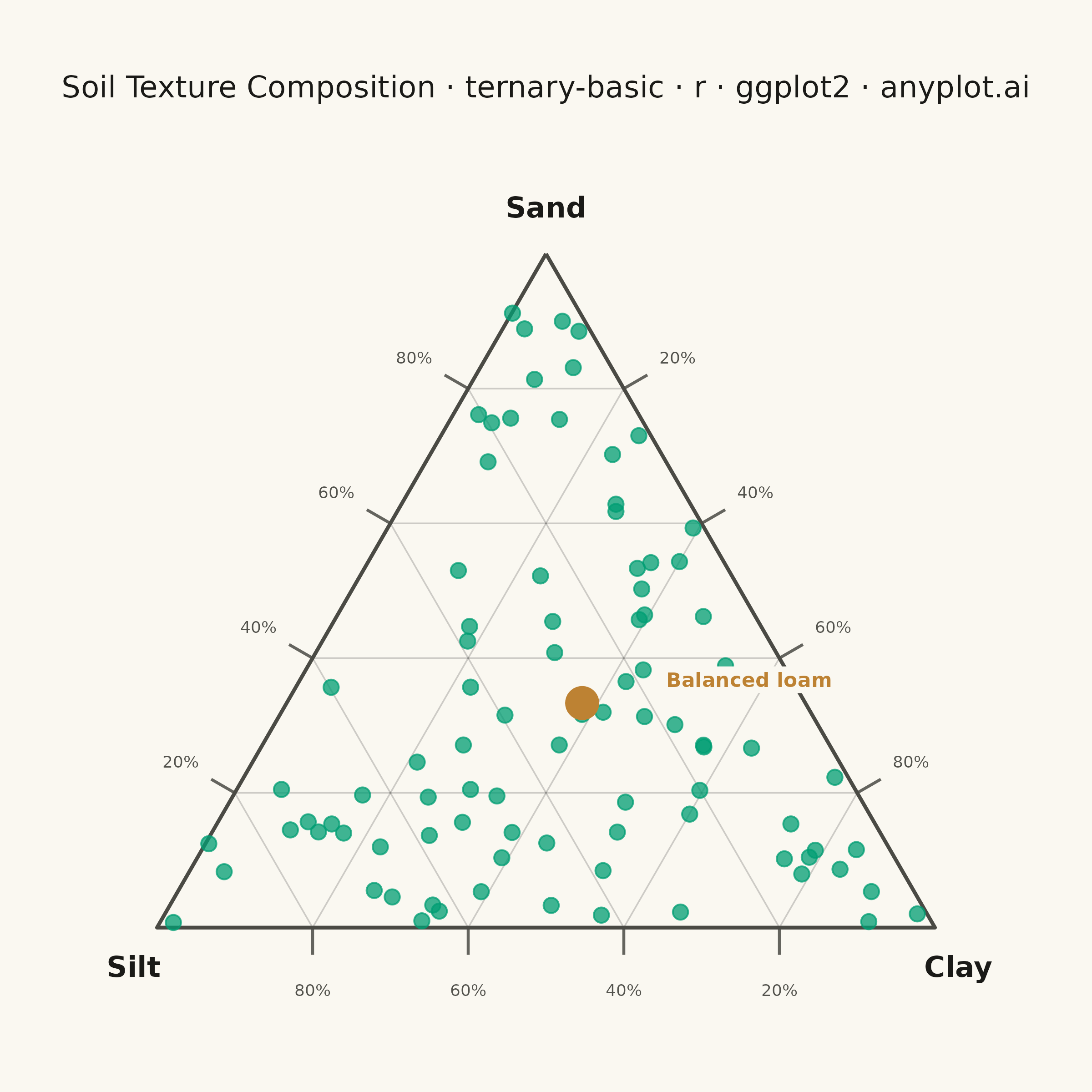
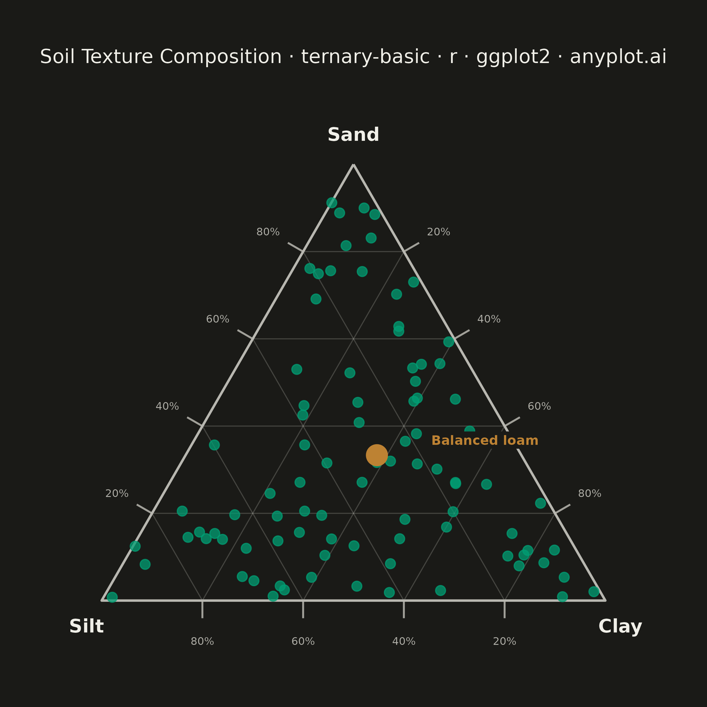
A ternary plot displays three-component compositional data on an equilateral triangle where each vertex represents 100% of one component. Points inside the triangle show compositions that sum to a constant total (usually 100%), with position indicating relative proportions. This visualization is essential for data where three variables are interdependent and constrained to sum to a fixed value.
#' anyplot.ai
#' ternary-basic: Basic Ternary Plot
#' Library: ggplot2 3.5.1 | R 4.4.1
#' Quality: 92/100 | Created: 2026-08-04

library(ggplot2)
library(dplyr)
library(tibble)
library(ragg)

set.seed(42)

# --- Theme tokens -------------------------------------------------------
THEME       <- Sys.getenv("ANYPLOT_THEME", "light")
PAGE_BG     <- if (THEME == "light") "#FAF8F1" else "#1A1A17"
INK         <- if (THEME == "light") "#1A1A17" else "#F0EFE8"
INK_SOFT    <- if (THEME == "light") "#4A4A44" else "#B8B7B0"
IMPRINT_PALETTE <- c("#009E73", "#C475FD", "#4467A3", "#BD8233",
                     "#AE3030", "#2ABCCD", "#954477", "#99B314")
BRAND <- IMPRINT_PALETTE[1]

# --- Data: soil texture samples (sand / silt / clay, % sum to 100) ------
n_samples <- 90
sand_raw <- -log(runif(n_samples))
silt_raw <- -log(runif(n_samples))
clay_raw <- -log(runif(n_samples))
total_raw <- sand_raw + silt_raw + clay_raw

soil <- tibble(
  sand = sand_raw / total_raw,
  silt = silt_raw / total_raw,
  clay = clay_raw / total_raw
) %>%
  mutate(
    x = clay + 0.5 * sand,
    y = sand * sqrt(3) / 2,
    balance_dist = sqrt((sand - 1 / 3)^2 + (silt - 1 / 3)^2 + (clay - 1 / 3)^2)
  )

# Focal point: the sample closest to an even 1/3-1/3-1/3 split ("balanced loam")
balanced_sample <- soil %>% slice_min(balance_dist, n = 1)

# --- Ternary scaffold: triangle border, grid lines, edge ticks ----------
# Barycentric layout: sand -> top vertex, silt -> bottom-left, clay -> bottom-right
vertices <- tibble(
  x     = c(0.5, 0, 1),
  y     = c(sqrt(3) / 2, 0, 0),
  label = c("Sand", "Silt", "Clay")
)
triangle_outline <- bind_rows(vertices, vertices[1, ])

grid_fracs <- seq(0.2, 0.8, by = 0.2)

grid_lines <- bind_rows(
  # constant sand (parallel to the Silt-Clay bottom edge)
  tibble(
    x    = 0.5 * grid_fracs,
    y    = grid_fracs * sqrt(3) / 2,
    xend = 1 - 0.5 * grid_fracs,
    yend = grid_fracs * sqrt(3) / 2
  ),
  # constant silt (parallel to the Sand-Clay edge)
  tibble(
    x    = 0.5 * (1 - grid_fracs),
    y    = (1 - grid_fracs) * sqrt(3) / 2,
    xend = 1 - grid_fracs,
    yend = 0
  ),
  # constant clay (parallel to the Sand-Silt edge)
  tibble(
    x    = 0.5 + 0.5 * grid_fracs,
    y    = (1 - grid_fracs) * sqrt(3) / 2,
    xend = grid_fracs,
    yend = 0
  )
)

tick_len <- 0.035
edge_ticks <- bind_rows(
  # bottom edge (Silt-Clay), ticks point straight down
  tibble(x = grid_fracs, y = 0, xend = grid_fracs, yend = -tick_len),
  # left edge (Sand-Silt), ticks point out to the upper-left
  tibble(
    x    = 0.5 * grid_fracs, y = grid_fracs * sqrt(3) / 2,
    xend = 0.5 * grid_fracs - tick_len * sqrt(3) / 2,
    yend = grid_fracs * sqrt(3) / 2 + tick_len * 0.5
  ),
  # right edge (Sand-Clay), ticks point out to the upper-right
  tibble(
    x    = 1 - 0.5 * grid_fracs, y = grid_fracs * sqrt(3) / 2,
    xend = 1 - 0.5 * grid_fracs + tick_len * sqrt(3) / 2,
    yend = grid_fracs * sqrt(3) / 2 + tick_len * 0.5
  )
)

# Percentage labels beyond each tick — one component scale per edge, each
# verified against the barycentric mapping so every edge reads a different,
# non-redundant value: bottom = Silt (x = clay when sand = 0, so silt = 1-x),
# left = Sand (y = sand*sqrt(3)/2 everywhere), right = Clay (silt = 0, so
# clay = 1 - sand there).
label_gap <- 0.045
edge_labels <- bind_rows(
  tibble(
    x = grid_fracs, y = -tick_len - label_gap,
    label = paste0(round((1 - grid_fracs) * 100), "%")
  ),
  tibble(
    x = 0.5 * grid_fracs - (tick_len + label_gap) * sqrt(3) / 2,
    y = grid_fracs * sqrt(3) / 2 + (tick_len + label_gap) * 0.5,
    label = paste0(round(grid_fracs * 100), "%")
  ),
  tibble(
    x = 1 - 0.5 * grid_fracs + (tick_len + label_gap) * sqrt(3) / 2,
    y = grid_fracs * sqrt(3) / 2 + (tick_len + label_gap) * 0.5,
    label = paste0(round((1 - grid_fracs) * 100), "%")
  )
)

# --- Title (fontsize scales down for titles longer than the 67-char baseline)
plot_title <- "Soil Texture Composition · ternary-basic · r · ggplot2 · anyplot.ai"
title_ratio <- if (nchar(plot_title) > 67) 67 / nchar(plot_title) else 1.0
title_size <- max(8, round(12 * title_ratio))

# --- Plot -----------------------------------------------------------------
p <- ggplot() +
  geom_segment(
    data = grid_lines, aes(x = x, y = y, xend = xend, yend = yend),
    color = INK, alpha = 0.2, linewidth = 0.3
  ) +
  geom_segment(
    data = edge_ticks, aes(x = x, y = y, xend = xend, yend = yend),
    color = INK_SOFT, alpha = 0.85, linewidth = 0.55
  ) +
  geom_text(
    data = edge_labels, aes(x = x, y = y, label = label),
    color = INK_SOFT, size = 2.3, alpha = 0.95
  ) +
  geom_path(
    data = triangle_outline, aes(x = x, y = y),
    color = INK_SOFT, linewidth = 0.7
  ) +
  geom_point(
    data = soil, aes(x = x, y = y),
    color = BRAND, size = 2.5, alpha = 0.75
  ) +
  geom_point(
    data = balanced_sample, aes(x = x, y = y),
    color = IMPRINT_PALETTE[4], fill = IMPRINT_PALETTE[4],
    shape = 21, size = 5, stroke = 1
  ) +
  geom_label(
    data = balanced_sample,
    aes(x = x + 0.1, y = y + 0.03, label = "Balanced loam"),
    color = IMPRINT_PALETTE[4], fill = PAGE_BG, label.size = 0,
    size = 2.8, fontface = "bold", hjust = 0
  ) +
  geom_text(
    data = vertices %>% mutate(
      y_offset = y + c(0.06, -0.05, -0.05),
      x_offset = x + c(0, -0.03, 0.03)
    ),
    aes(x = x_offset, y = y_offset, label = label),
    color = INK, size = 4, fontface = "bold"
  ) +
  labs(title = plot_title) +
  coord_fixed(ratio = 1, xlim = c(-0.15, 1.15), ylim = c(-0.14, 1.02), expand = FALSE) +
  theme_void(base_size = 8) +
  theme(
    plot.background = element_rect(fill = PAGE_BG, color = PAGE_BG),
    panel.background = element_rect(fill = PAGE_BG, color = NA),
    plot.title = element_text(
      color = INK, size = title_size, face = "plain",
      hjust = 0.5, margin = margin(b = 12)
    ),
    plot.margin = margin(t = 16, r = 16, b = 8, l = 16)
  )

# --- Save -------------------------------------------------------------------
ggsave(
  filename = sprintf("plot-%s.png", THEME),
  plot     = p,
  device   = ragg::agg_png,
  width    = 6,
  height   = 6,
  units    = "in",
  dpi      = 400
)
Runnable source as JSON, for any HTTP client: https://api.anyplot.ai/specs/ternary-basic/ggplot2/code. Any spec id and library id listed in llms-full.txt fit the same URL shape; every URL below is complete and callable.
{
  "spec_id": "ternary-basic",
  "language": "r",
  "library": "ggplot2",
  "page": "https://anyplot.ai/ternary-basic/r/ggplot2",
  "hub": "https://anyplot.ai/ternary-basic",
  "code_json": "https://api.anyplot.ai/specs/ternary-basic/ggplot2/code",
  "spec_json": "https://api.anyplot.ai/specs/ternary-basic",
  "render_light_png": "https://storage.googleapis.com/anyplot-images/plots/ternary-basic/r/ggplot2/plot-light.png",
  "render_dark_png": "https://storage.googleapis.com/anyplot-images/plots/ternary-basic/r/ggplot2/plot-dark.png",
  "quality_score": 92.0,
  "license": "MIT",
  "guide": "https://anyplot.ai/llms.txt"
}
Part of Basic Ternary Plot on anyplot.ai.