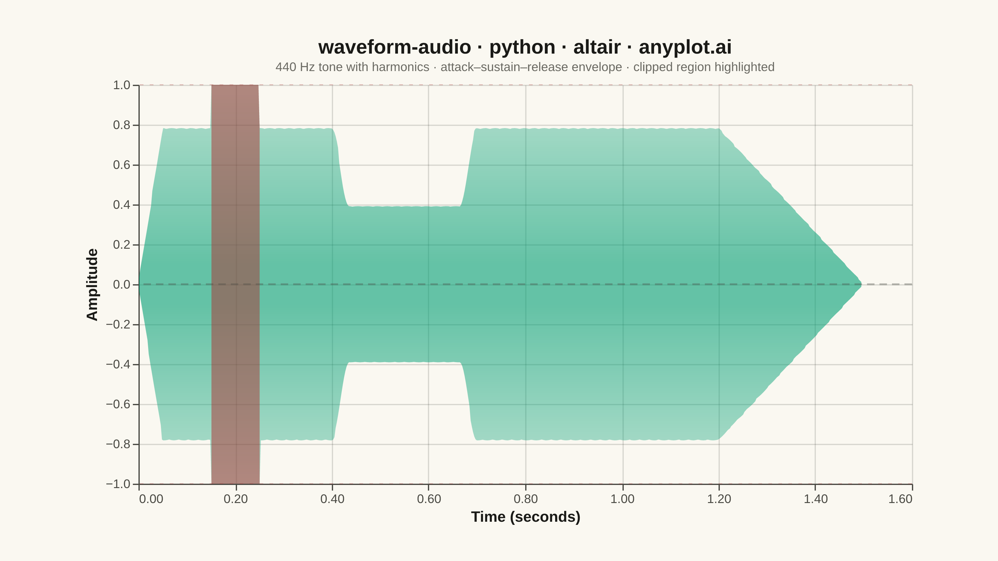
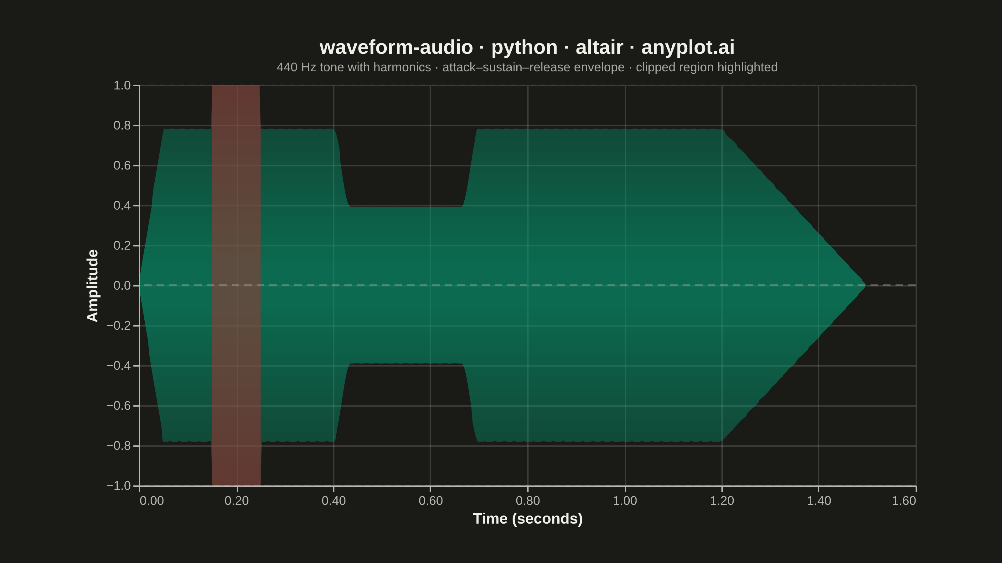
A time-domain visualization of audio amplitude that displays the raw waveform shape as seen in digital audio workstations (DAWs). The plot shows positive and negative amplitude symmetrically around a zero baseline, with time on the x-axis and normalized amplitude (-1 to +1) on the y-axis. This is the fundamental representation for inspecting audio signals, revealing dynamics, clipping, silence, and transient characteristics at a glance.
""" anyplot.ai
waveform-audio: Audio Waveform Plot
Library: altair 6.1.0 | Python 3.13.13
Quality: 92/100 | Updated: 2026-06-03
"""

import os

import altair as alt
import numpy as np
import pandas as pd
from PIL import Image


THEME = os.getenv("ANYPLOT_THEME", "light")
PAGE_BG = "#FAF8F1" if THEME == "light" else "#1A1A17"
ELEVATED_BG = "#FFFDF6" if THEME == "light" else "#242420"
INK = "#1A1A17" if THEME == "light" else "#F0EFE8"
INK_SOFT = "#4A4A44" if THEME == "light" else "#B8B7B0"
INK_MUTED = "#6B6A63" if THEME == "light" else "#A8A79F"

# Imprint palette — semantic anchor for clipping regions
CLIP_COLOR = "#AE3030"  # matte red: error/clipping role

# Data - synthetic audio: 440 Hz tone with harmonics and amplitude envelope
sample_rate = 22050
duration = 1.5
num_samples = int(sample_rate * duration)
time = np.linspace(0, duration, num_samples)

fundamental = 440
signal = (
    0.6 * np.sin(2 * np.pi * fundamental * time)
    + 0.25 * np.sin(2 * np.pi * 2 * fundamental * time)
    + 0.15 * np.sin(2 * np.pi * 3 * fundamental * time)
)

# Attack-sustain-release envelope with amplitude dip and brief clipping boost
envelope = np.ones_like(time)
attack = int(0.05 * sample_rate)
release = int(0.3 * sample_rate)
envelope[:attack] = np.linspace(0, 1, attack)
envelope[-release:] = np.linspace(1, 0, release)

# Smooth amplitude dip (0.4-0.7 s) via cosine taper — avoids abrupt rectangular step
dip_start = int(0.4 * sample_rate)
dip_end = int(0.7 * sample_rate)
transition_len = int(0.035 * sample_rate)
t_fade = np.linspace(0, 1, transition_len)
dip_mult = np.ones_like(time)
dip_mult[dip_start : dip_start + transition_len] = 1.0 - 0.25 * (1 - np.cos(np.pi * t_fade))
dip_mult[dip_start + transition_len : dip_end - transition_len] = 0.5
dip_mult[dip_end - transition_len : dip_end] = 0.5 + 0.25 * (1 - np.cos(np.pi * t_fade))
envelope *= dip_mult

envelope[int(0.15 * sample_rate) : int(0.25 * sample_rate)] *= 1.35

signal = signal * envelope
signal = np.clip(signal, -1.0, 1.0)

# Min/max envelope binning — 600 bins avoids sub-pixel vertical striping artifacts
num_bins = 600
bin_size = num_samples // num_bins
usable = num_bins * bin_size
signal_trimmed = signal[:usable].reshape(num_bins, bin_size)
time_trimmed = time[:usable].reshape(num_bins, bin_size)

df = pd.DataFrame(
    {
        "time": time_trimmed[:, bin_size // 2],
        "amp_min": signal_trimmed.min(axis=1),
        "amp_max": signal_trimmed.max(axis=1),
    }
)
df["clipped"] = (df["amp_max"] >= 0.99) | (df["amp_min"] <= -0.99)

# Shared encodings
x_enc = alt.X("time:Q", title="Time (seconds)", axis=alt.Axis(format=".2f", tickCount=8))
y_enc = alt.Y("amp_min:Q", title="Amplitude", scale=alt.Scale(domain=[-1.0, 1.0]))

# Nearest-point selection for interactive crosshair
nearest = alt.selection_point(nearest=True, on="pointerover", fields=["time"], empty=False)

# Main waveform: Imprint brand green (#009E73) vertical gradient
waveform_gradient = (
    alt.Chart(df)
    .mark_area(
        interpolate="linear",
        color=alt.Gradient(
            gradient="linear",
            stops=[
                alt.GradientStop(color="rgba(0, 158, 115, 0.28)", offset=0),
                alt.GradientStop(color="rgba(0, 158, 115, 0.60)", offset=0.45),
                alt.GradientStop(color="rgba(0, 158, 115, 0.60)", offset=0.55),
                alt.GradientStop(color="rgba(0, 158, 115, 0.28)", offset=1),
            ],
            x1=0,
            x2=0,
            y1=0,
            y2=1,
        ),
        line=False,
    )
    .encode(x=x_enc, y=y_enc, y2="amp_max:Q")
)

# Clipped regions overlay — Imprint matte red (#AE3030) semantic anchor
clipped_overlay = (
    alt.Chart(df)
    .mark_area(interpolate="linear", color="rgba(174, 48, 48, 0.50)", line=False)
    .encode(x="time:Q", y=y_enc, y2="amp_max:Q")
    .transform_filter(alt.datum.clipped == True)
)

# Zero baseline reference line (theme-adaptive)
zero_line = (
    alt.Chart(pd.DataFrame({"y": [0]}))
    .mark_rule(strokeWidth=1.5, opacity=0.35, strokeDash=[6, 4])
    .encode(y="y:Q", color=alt.value(INK_SOFT))
)

# Clipping threshold lines at ±1.0 (semantic matte red)
clip_lines = (
    alt.Chart(pd.DataFrame({"y": [-1.0, 1.0]}))
    .mark_rule(strokeWidth=0.8, opacity=0.3, strokeDash=[3, 5])
    .encode(y="y:Q", color=alt.value(CLIP_COLOR))
)

# Interactive crosshair following pointer
crosshair_rule = (
    alt.Chart(df)
    .mark_rule(strokeWidth=1, opacity=0.5)
    .encode(x="time:Q", color=alt.value(INK_SOFT))
    .transform_filter(nearest)
)

# Invisible selection trigger with tooltips
selection_layer = (
    alt.Chart(df)
    .mark_point(opacity=0)
    .encode(
        x="time:Q",
        y="amp_max:Q",
        tooltip=[
            alt.Tooltip("time:Q", title="Time (s)", format=".3f"),
            alt.Tooltip("amp_max:Q", title="Peak", format=".3f"),
            alt.Tooltip("amp_min:Q", title="Trough", format=".3f"),
        ],
    )
    .add_params(nearest)
)

# Compose layers and apply theme-adaptive configuration
chart = (
    alt.layer(waveform_gradient, clipped_overlay, zero_line, clip_lines, crosshair_rule, selection_layer)
    .properties(
        width=620,
        height=320,
        background=PAGE_BG,
        title=alt.Title(
            "waveform-audio · python · altair · anyplot.ai",
            fontSize=16,
            subtitle="440 Hz tone with harmonics · attack–sustain–release envelope · clipped region highlighted",
            subtitleFontSize=10,
        ),
    )
    .configure_view(fill=PAGE_BG, strokeWidth=0, continuousWidth=620, continuousHeight=320)
    .configure_axis(
        labelFontSize=10,
        titleFontSize=12,
        gridColor=INK,
        gridOpacity=0.15,
        domainColor=INK_SOFT,
        tickColor=INK_SOFT,
        labelColor=INK_SOFT,
        titleColor=INK,
    )
    .configure_title(color=INK, subtitleColor=INK_MUTED)
)

# Save PNG and pad to exact 3200×1800 (landscape target)
chart.save(f"plot-{THEME}.png", scale_factor=4.0)

TW, TH = 3200, 1800
_img = Image.open(f"plot-{THEME}.png").convert("RGB")
_w, _h = _img.size
if _w > TW or _h > TH:
    raise SystemExit(
        f"altair vl-convert produced {_w}×{_h}, exceeds target {TW}×{TH}. "
        "Shrink chart .properties(width=, height=) values and re-render."
    )
if _w < TW or _h < TH:
    _canvas = Image.new("RGB", (TW, TH), PAGE_BG)
    _canvas.paste(_img, ((TW - _w) // 2, (TH - _h) // 2))
    _canvas.save(f"plot-{THEME}.png")

# Save interactive HTML
chart.interactive().save(f"plot-{THEME}.html")
Runnable source as JSON, for any HTTP client: https://api.anyplot.ai/specs/waveform-audio/altair/code. Any spec id and library id listed in llms-full.txt fit the same URL shape; every URL below is complete and callable.
{
  "spec_id": "waveform-audio",
  "language": "python",
  "library": "altair",
  "page": "https://anyplot.ai/waveform-audio/python/altair",
  "hub": "https://anyplot.ai/waveform-audio",
  "code_json": "https://api.anyplot.ai/specs/waveform-audio/altair/code",
  "spec_json": "https://api.anyplot.ai/specs/waveform-audio",
  "render_light_png": "https://storage.googleapis.com/anyplot-images/plots/waveform-audio/python/altair/plot-light.png",
  "render_dark_png": "https://storage.googleapis.com/anyplot-images/plots/waveform-audio/python/altair/plot-dark.png",
  "interactive_light_html": "https://storage.googleapis.com/anyplot-images/plots/waveform-audio/python/altair/plot-light.html",
  "interactive_dark_html": "https://storage.googleapis.com/anyplot-images/plots/waveform-audio/python/altair/plot-dark.html",
  "quality_score": 92.0,
  "license": "MIT",
  "guide": "https://anyplot.ai/llms.txt"
}
Part of Audio Waveform Plot on anyplot.ai.