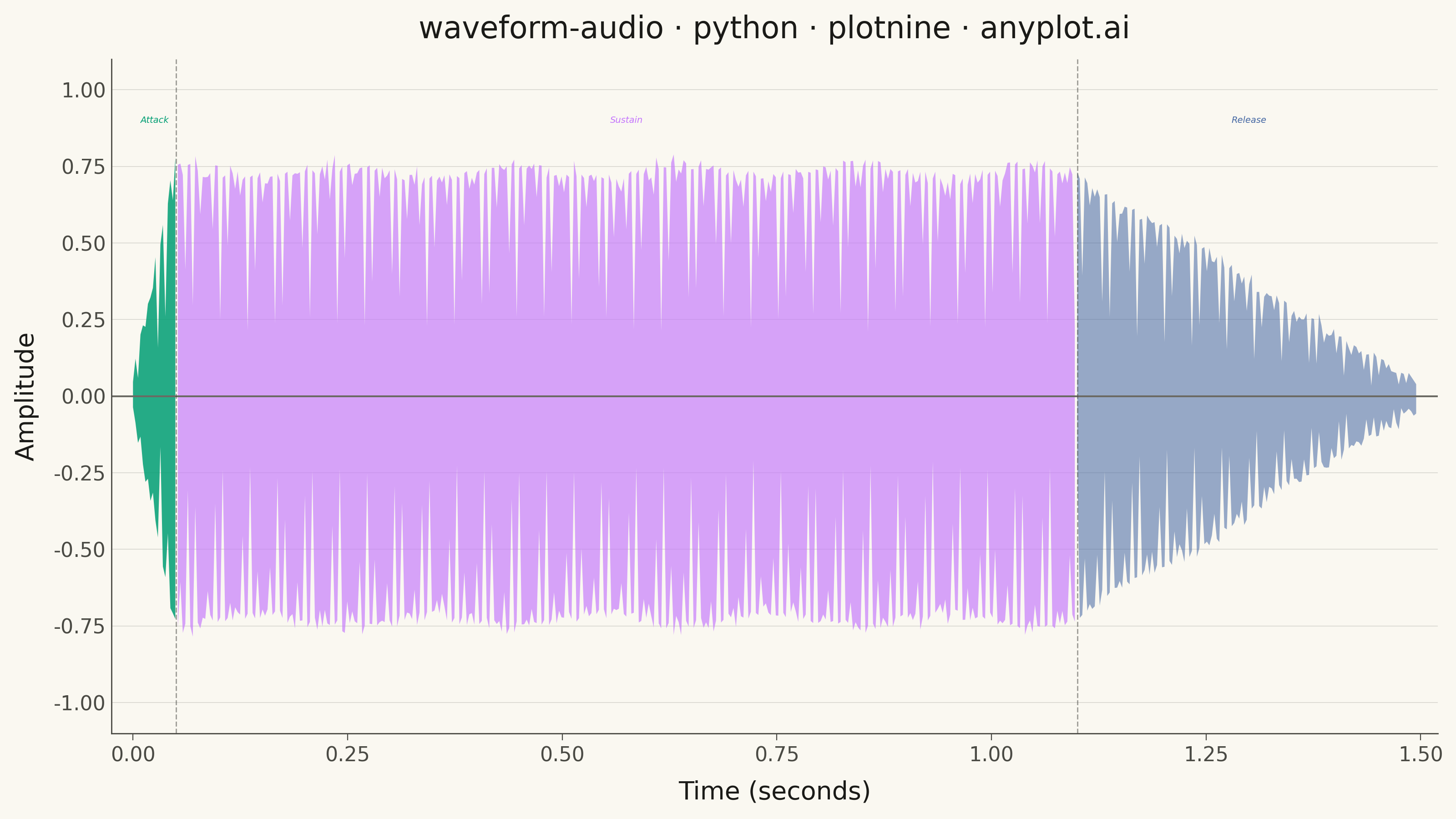
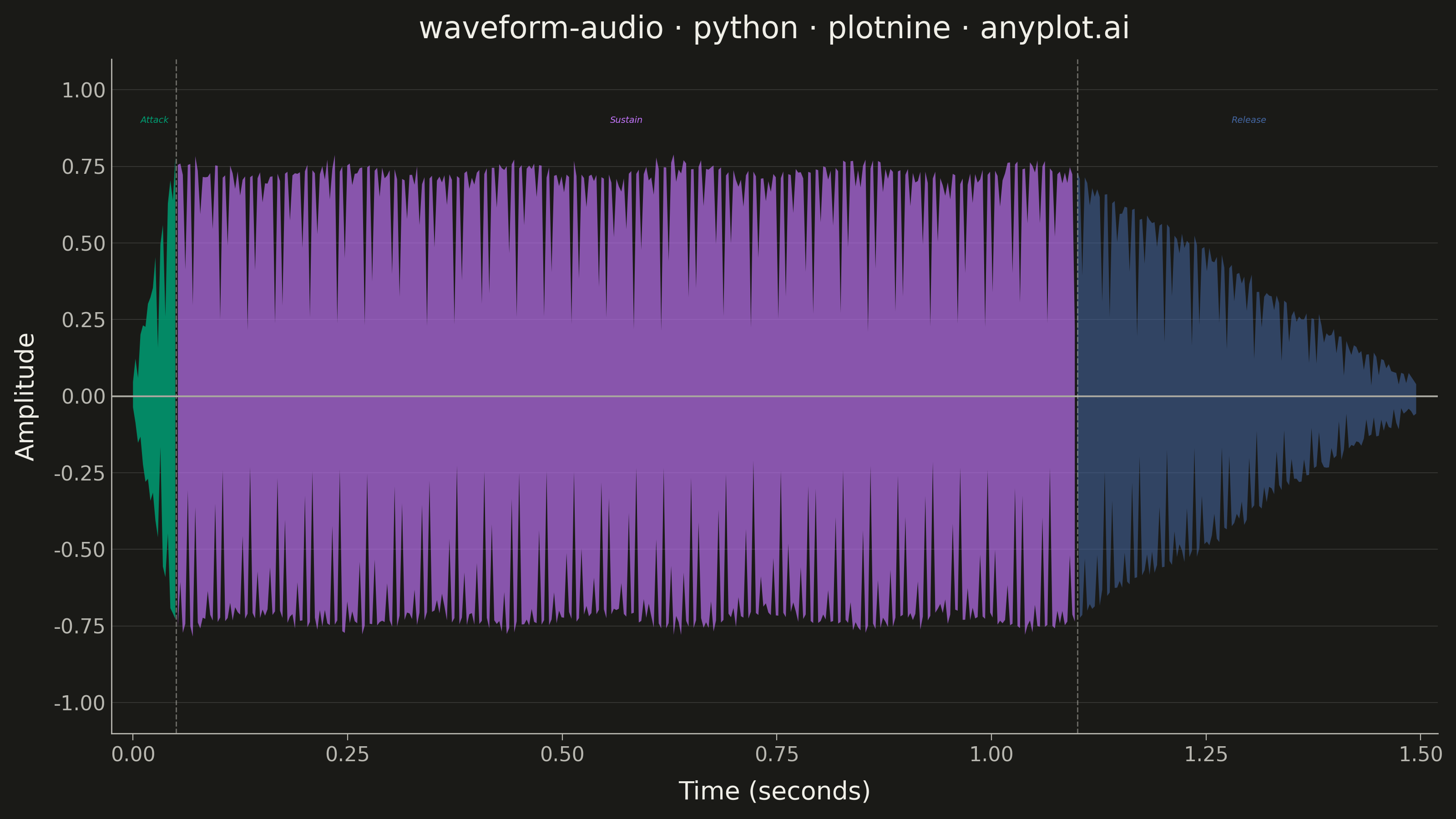
A time-domain visualization of audio amplitude that displays the raw waveform shape as seen in digital audio workstations (DAWs). The plot shows positive and negative amplitude symmetrically around a zero baseline, with time on the x-axis and normalized amplitude (-1 to +1) on the y-axis. This is the fundamental representation for inspecting audio signals, revealing dynamics, clipping, silence, and transient characteristics at a glance.
""" anyplot.ai
waveform-audio: Audio Waveform Plot
Library: plotnine 0.15.5 | Python 3.13.13
Quality: 86/100 | Updated: 2026-06-03
"""

import os

import numpy as np
import pandas as pd
from plotnine import (
    aes,
    annotate,
    element_blank,
    element_line,
    element_rect,
    element_text,
    geom_hline,
    geom_ribbon,
    geom_vline,
    ggplot,
    labs,
    scale_alpha_manual,
    scale_fill_manual,
    scale_x_continuous,
    scale_y_continuous,
    theme,
    theme_minimal,
)


# Theme tokens
THEME = os.getenv("ANYPLOT_THEME", "light")
PAGE_BG = "#FAF8F1" if THEME == "light" else "#1A1A17"
INK = "#1A1A17" if THEME == "light" else "#F0EFE8"
INK_SOFT = "#4A4A44" if THEME == "light" else "#B8B7B0"
INK_MUTED = "#6B6A63" if THEME == "light" else "#A8A79F"

# Imprint palette — positions 1, 2, 3 for Attack, Sustain, Release phases
IMPRINT_PALETTE = ["#009E73", "#C475FD", "#4467A3", "#BD8233", "#AE3030", "#2ABCCD", "#954477", "#99B314"]

# Data - synthetic audio waveform: tone with harmonics and amplitude envelope
np.random.seed(42)
sample_rate = 22050
duration = 1.5
num_samples = int(sample_rate * duration)
time = np.linspace(0, duration, num_samples)

fundamental = 220
signal = (
    0.6 * np.sin(2 * np.pi * fundamental * time)
    + 0.25 * np.sin(2 * np.pi * fundamental * 2 * time)
    + 0.1 * np.sin(2 * np.pi * fundamental * 3 * time)
    + 0.05 * np.sin(2 * np.pi * fundamental * 5 * time)
)

envelope = np.ones_like(time)
attack_end = int(0.05 * sample_rate)
sustain_end = int(1.1 * sample_rate)
envelope[:attack_end] = np.linspace(0, 1, attack_end)
envelope[sustain_end:] = np.linspace(1, 0, num_samples - sustain_end)

vibrato = 1.0 + 0.03 * np.sin(2 * np.pi * 5 * time)
noise = np.random.normal(0, 0.02, num_samples)
amplitude = np.clip((signal * envelope * vibrato) + noise, -1.0, 1.0)

# Downsample using min/max envelope to avoid aliasing
chunk_size = 64
num_chunks = num_samples // chunk_size
time_chunks = np.array([time[i * chunk_size] for i in range(num_chunks)])
amp_min = np.array([amplitude[i * chunk_size : (i + 1) * chunk_size].min() for i in range(num_chunks)])
amp_max = np.array([amplitude[i * chunk_size : (i + 1) * chunk_size].max() for i in range(num_chunks)])

attack_time = 0.05
sustain_time = 1.1
phase = []
for t in time_chunks:
    if t < attack_time:
        phase.append("Attack")
    elif t < sustain_time:
        phase.append("Sustain")
    else:
        phase.append("Release")

df = pd.DataFrame(
    {
        "time": time_chunks,
        "amp_min": amp_min,
        "amp_max": amp_max,
        "phase": pd.Categorical(phase, categories=["Attack", "Sustain", "Release"], ordered=True),
    }
)

# Imprint palette: Attack=green (pos 1), Sustain=lavender (pos 2), Release=blue (pos 3)
phase_colors = {"Attack": IMPRINT_PALETTE[0], "Sustain": IMPRINT_PALETTE[1], "Release": IMPRINT_PALETTE[2]}
phase_alphas = {"Attack": 0.85, "Sustain": 0.65, "Release": 0.55}

title = "waveform-audio · python · plotnine · anyplot.ai"

# Plot
plot = (
    ggplot(df, aes(x="time"))
    + geom_ribbon(aes(ymin="amp_min", ymax="amp_max", fill="phase", alpha="phase"), show_legend=False)
    + scale_fill_manual(values=phase_colors)
    + scale_alpha_manual(values=phase_alphas)
    + geom_hline(yintercept=0, color=INK_MUTED, size=0.4, linetype="solid")
    + geom_vline(xintercept=attack_time, color=INK_SOFT, size=0.3, linetype="dashed", alpha=0.5)
    + geom_vline(xintercept=sustain_time, color=INK_SOFT, size=0.3, linetype="dashed", alpha=0.5)
    + annotate("text", x=0.025, y=0.90, label="Attack", size=3.5, color=IMPRINT_PALETTE[0], fontstyle="italic")
    + annotate("text", x=0.575, y=0.90, label="Sustain", size=3.5, color=IMPRINT_PALETTE[1], fontstyle="italic")
    + annotate("text", x=1.30, y=0.90, label="Release", size=3.5, color=IMPRINT_PALETTE[2], fontstyle="italic")
    + labs(x="Time (seconds)", y="Amplitude", title=title)
    + scale_x_continuous(
        breaks=np.arange(0, duration + 0.1, 0.25), labels=lambda lst: [f"{v:.2f}" for v in lst], expand=(0.01, 0.01)
    )
    + scale_y_continuous(limits=(-1.0, 1.0), breaks=np.arange(-1.0, 1.1, 0.25))
    + theme_minimal()
    + theme(
        figure_size=(8, 4.5),
        text=element_text(size=7, color=INK),
        axis_title=element_text(size=10, color=INK),
        axis_text=element_text(size=8, color=INK_SOFT),
        plot_title=element_text(size=12, color=INK),
        legend_text=element_text(size=8, color=INK_SOFT),
        panel_background=element_rect(fill=PAGE_BG, color="none"),
        plot_background=element_rect(fill=PAGE_BG, color="none"),
        panel_grid_major_y=element_line(color=INK, size=0.3, alpha=0.15),
        panel_grid_major_x=element_blank(),
        panel_grid_minor=element_blank(),
        axis_line_x=element_line(color=INK_SOFT, size=0.5),
        axis_line_y=element_line(color=INK_SOFT, size=0.5),
        axis_ticks_major_x=element_line(color=INK_SOFT, size=0.4),
        axis_ticks_major_y=element_blank(),
    )
)

plot.save(f"plot-{THEME}.png", dpi=400, width=8, height=4.5, units="in", verbose=False)
Runnable source as JSON, for any HTTP client: https://api.anyplot.ai/specs/waveform-audio/plotnine/code. Any spec id and library id listed in llms-full.txt fit the same URL shape; every URL below is complete and callable.
{
  "spec_id": "waveform-audio",
  "language": "python",
  "library": "plotnine",
  "page": "https://anyplot.ai/waveform-audio/python/plotnine",
  "hub": "https://anyplot.ai/waveform-audio",
  "code_json": "https://api.anyplot.ai/specs/waveform-audio/plotnine/code",
  "spec_json": "https://api.anyplot.ai/specs/waveform-audio",
  "render_light_png": "https://storage.googleapis.com/anyplot-images/plots/waveform-audio/python/plotnine/plot-light.png",
  "render_dark_png": "https://storage.googleapis.com/anyplot-images/plots/waveform-audio/python/plotnine/plot-dark.png",
  "quality_score": 86.0,
  "license": "MIT",
  "guide": "https://anyplot.ai/llms.txt"
}
Part of Audio Waveform Plot on anyplot.ai.