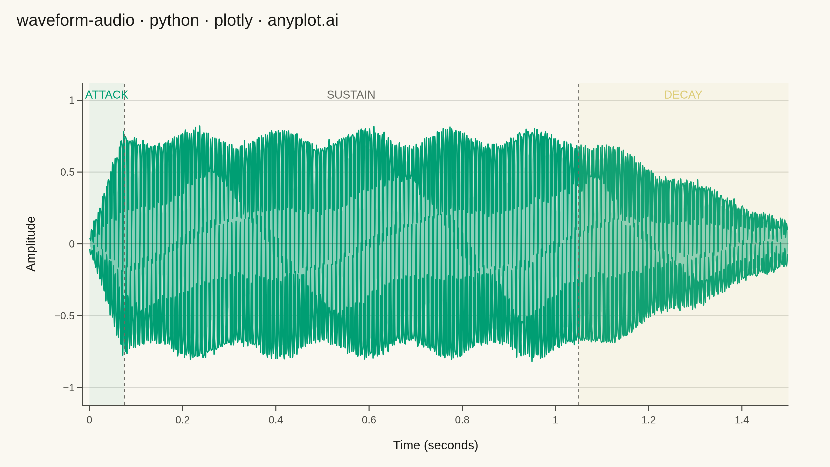
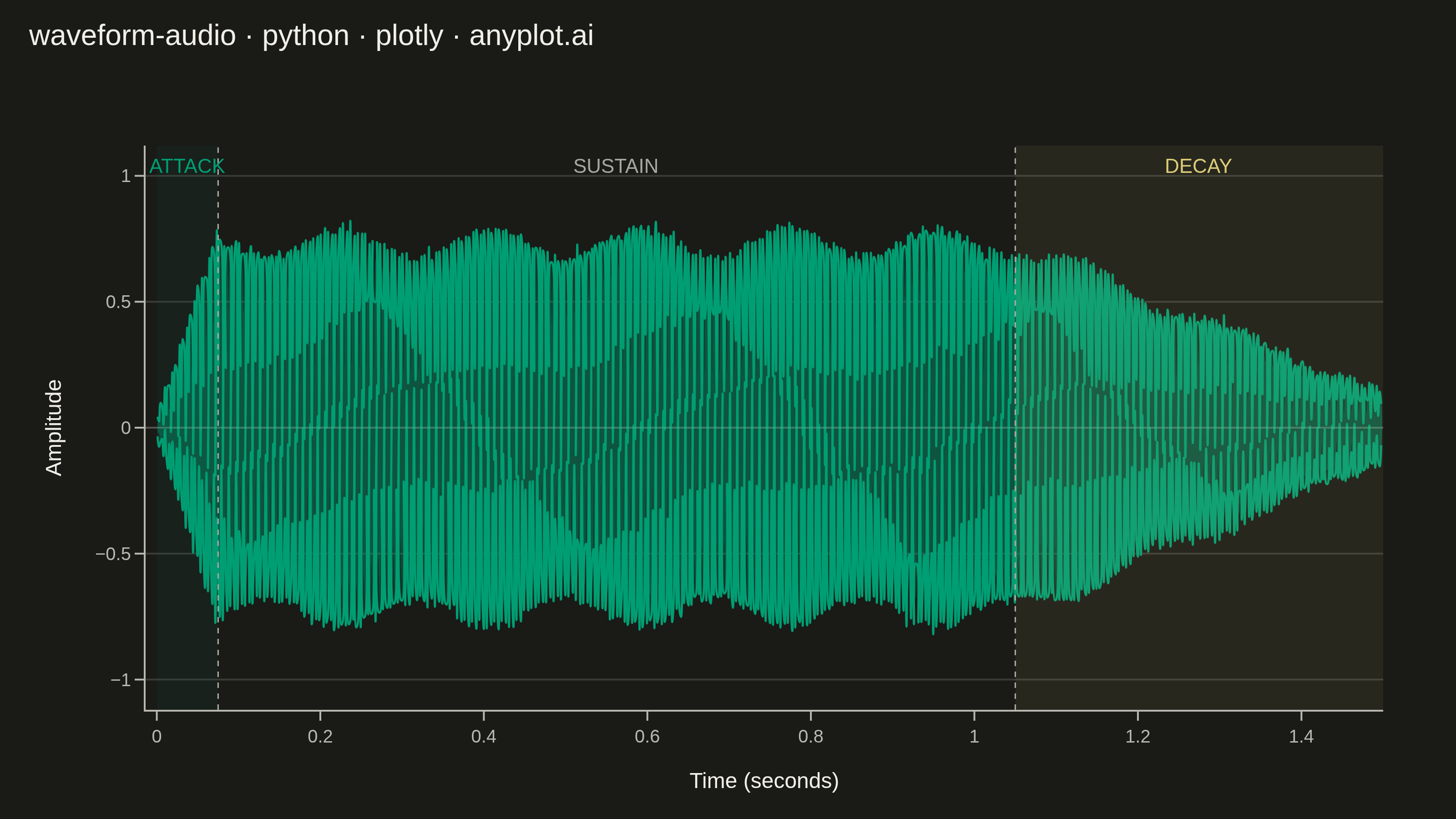
A time-domain visualization of audio amplitude that displays the raw waveform shape as seen in digital audio workstations (DAWs). The plot shows positive and negative amplitude symmetrically around a zero baseline, with time on the x-axis and normalized amplitude (-1 to +1) on the y-axis. This is the fundamental representation for inspecting audio signals, revealing dynamics, clipping, silence, and transient characteristics at a glance.
""" anyplot.ai
waveform-audio: Audio Waveform Plot
Library: plotly 6.7.0 | Python 3.13.13
Quality: 92/100 | Updated: 2026-06-03
"""

import os
import sys


# Prevent self-import: remove this script's own directory from sys.path so that
# "import plotly" resolves to the installed package, not this file.
_here = os.path.dirname(os.path.abspath(__file__))
sys.path = [p for p in sys.path if os.path.abspath(p) != _here]

import numpy as np
import plotly.graph_objects as go


# Theme-adaptive chrome (Imprint palette)
THEME = os.getenv("ANYPLOT_THEME", "light")
PAGE_BG = "#FAF8F1" if THEME == "light" else "#1A1A17"
ELEVATED_BG = "#FFFDF6" if THEME == "light" else "#242420"
INK = "#1A1A17" if THEME == "light" else "#F0EFE8"
INK_SOFT = "#4A4A44" if THEME == "light" else "#B8B7B0"
INK_MUTED = "#6B6A63" if THEME == "light" else "#A8A79F"
GRID = "rgba(26,26,23,0.15)" if THEME == "light" else "rgba(240,239,232,0.15)"

# Imprint palette — first series is always #009E73
BRAND = "#009E73"
ANYPLOT_AMBER = "#DDCC77"  # warning / decay semantic role

# Data
np.random.seed(42)
sample_rate = 22050
duration = 1.5
num_samples = int(sample_rate * duration)
time = np.linspace(0, duration, num_samples)

# Synthesize audio: fundamental tone + harmonics with amplitude envelope
fundamental_freq = 220
signal = (
    0.6 * np.sin(2 * np.pi * fundamental_freq * time)
    + 0.25 * np.sin(2 * np.pi * fundamental_freq * 2 * time)
    + 0.1 * np.sin(2 * np.pi * fundamental_freq * 3 * time)
    + 0.05 * np.sin(2 * np.pi * fundamental_freq * 5 * time)
)

# Amplitude envelope: attack-sustain-decay shape
envelope = np.ones_like(time)
attack_end = int(0.05 * num_samples)
decay_start = int(0.7 * num_samples)
envelope[:attack_end] = np.linspace(0, 1, attack_end)
envelope[decay_start:] = np.linspace(1, 0.15, num_samples - decay_start)

# Slight tremolo and noise for realism
tremolo = 1.0 + 0.08 * np.sin(2 * np.pi * 5.5 * time)
amplitude = signal * envelope * tremolo
amplitude += np.random.normal(0, 0.02, num_samples)
amplitude = np.clip(amplitude, -1.0, 1.0)

# Downsample with larger blocks for cleaner sustain region visibility
block_size = 40
num_blocks = num_samples // block_size
time_blocks = np.array([(time[i * block_size] + time[(i + 1) * block_size - 1]) / 2 for i in range(num_blocks)])
amp_max = np.array([amplitude[i * block_size : (i + 1) * block_size].max() for i in range(num_blocks)])
amp_min = np.array([amplitude[i * block_size : (i + 1) * block_size].min() for i in range(num_blocks)])

# Data-derived inner envelope: 70th percentile of absolute amplitude per block
# Captures the RMS-like energy content rather than an arbitrary fixed scaling factor
amp_p70 = np.array(
    [np.percentile(np.abs(amplitude[i * block_size : (i + 1) * block_size]), 70) for i in range(num_blocks)]
)

# Phase boundaries
attack_time = duration * 0.05
decay_time = duration * 0.7

# Plot
fig = go.Figure()

# Outer waveform envelope (Imprint brand green fill)
fig.add_trace(
    go.Scatter(
        x=np.concatenate([time_blocks, time_blocks[::-1]]),
        y=np.concatenate([amp_max, amp_min[::-1]]),
        fill="toself",
        fillcolor="rgba(0,158,115,0.18)",
        line={"color": "rgba(0,158,115,0.5)", "width": 0.5, "shape": "spline"},
        name="Waveform",
        hovertemplate="Time: %{x:.3f}s<br>Amplitude: %{y:.3f}<extra></extra>",
    )
)

# Inner envelope: data-derived 70th-percentile energy bounds for visual depth
fig.add_trace(
    go.Scatter(
        x=np.concatenate([time_blocks, time_blocks[::-1]]),
        y=np.concatenate([amp_p70, -amp_p70[::-1]]),
        fill="toself",
        fillcolor="rgba(0,158,115,0.32)",
        line={"width": 0, "shape": "spline"},
        showlegend=False,
        hoverinfo="skip",
    )
)

# Peak envelope lines for crisp edge definition
fig.add_trace(
    go.Scatter(
        x=time_blocks,
        y=amp_max,
        mode="lines",
        line={"color": BRAND, "width": 1.2, "shape": "spline"},
        showlegend=False,
        hoverinfo="skip",
    )
)
fig.add_trace(
    go.Scatter(
        x=time_blocks,
        y=amp_min,
        mode="lines",
        line={"color": BRAND, "width": 1.2, "shape": "spline"},
        showlegend=False,
        hoverinfo="skip",
    )
)

# Zero reference line
fig.add_hline(y=0, line_dash="solid", line_color=GRID, line_width=1)

# Phase region shading (subtle — semantic color cues, not data)
fig.add_vrect(x0=0, x1=attack_time, fillcolor="rgba(0,158,115,0.06)", line_width=0)
fig.add_vrect(x0=decay_time, x1=duration, fillcolor="rgba(221,204,119,0.08)", line_width=0)

# Phase boundary markers
for t_boundary in [attack_time, decay_time]:
    fig.add_vline(x=t_boundary, line_dash="dot", line_color=INK_MUTED, line_width=0.8)

# Phase annotations — semantic color coding: green=start, muted=stable, amber=fade
fig.add_annotation(
    x=attack_time / 2,
    y=1.04,
    text="ATTACK",
    showarrow=False,
    font={"size": 11, "color": BRAND, "family": "Arial Black, sans-serif"},
    yref="y",
)
fig.add_annotation(
    x=(attack_time + decay_time) / 2,
    y=1.04,
    text="SUSTAIN",
    showarrow=False,
    font={"size": 11, "color": INK_MUTED, "family": "Arial Black, sans-serif"},
    yref="y",
)
fig.add_annotation(
    x=(decay_time + duration) / 2,
    y=1.04,
    text="DECAY",
    showarrow=False,
    font={"size": 11, "color": ANYPLOT_AMBER, "family": "Arial Black, sans-serif"},
    yref="y",
)

# Layout with canonical canvas, theme-adaptive chrome, and correct font sizes
fig.update_layout(
    autosize=False,
    paper_bgcolor=PAGE_BG,
    plot_bgcolor=PAGE_BG,
    font={"color": INK},
    title={
        "text": "waveform-audio · python · plotly · anyplot.ai",
        "font": {"size": 16, "color": INK, "family": "Arial Black, sans-serif"},
        "x": 0.02,
        "xanchor": "left",
        "y": 0.97,
        "yanchor": "top",
    },
    xaxis={
        "title": {"text": "Time (seconds)", "font": {"size": 12, "color": INK}},
        "tickfont": {"size": 10, "color": INK_SOFT},
        "showgrid": False,
        "zeroline": False,
        "linecolor": INK_SOFT,
        "linewidth": 1,
        "ticks": "outside",
        "tickcolor": INK_SOFT,
        "ticklen": 5,
    },
    yaxis={
        "title": {"text": "Amplitude", "font": {"size": 12, "color": INK}},
        "tickfont": {"size": 10, "color": INK_SOFT},
        "range": [-1.12, 1.12],
        "showgrid": True,
        "gridcolor": GRID,
        "gridwidth": 1,
        "zeroline": False,
        "linecolor": INK_SOFT,
        "linewidth": 1,
        "ticks": "outside",
        "tickcolor": INK_SOFT,
        "ticklen": 5,
        "dtick": 0.5,
    },
    showlegend=False,
    margin={"l": 80, "r": 40, "t": 80, "b": 60},
)

# Save — canonical plotly landscape: width=800, height=450, scale=4 → 3200×1800 px
fig.write_image(f"plot-{THEME}.png", width=800, height=450, scale=4)
fig.write_html(f"plot-{THEME}.html", include_plotlyjs="cdn")
Runnable source as JSON, for any HTTP client: https://api.anyplot.ai/specs/waveform-audio/plotly/code. Any spec id and library id listed in llms-full.txt fit the same URL shape; every URL below is complete and callable.
{
  "spec_id": "waveform-audio",
  "language": "python",
  "library": "plotly",
  "page": "https://anyplot.ai/waveform-audio/python/plotly",
  "hub": "https://anyplot.ai/waveform-audio",
  "code_json": "https://api.anyplot.ai/specs/waveform-audio/plotly/code",
  "spec_json": "https://api.anyplot.ai/specs/waveform-audio",
  "render_light_png": "https://storage.googleapis.com/anyplot-images/plots/waveform-audio/python/plotly/plot-light.png",
  "render_dark_png": "https://storage.googleapis.com/anyplot-images/plots/waveform-audio/python/plotly/plot-dark.png",
  "interactive_light_html": "https://storage.googleapis.com/anyplot-images/plots/waveform-audio/python/plotly/plot-light.html",
  "interactive_dark_html": "https://storage.googleapis.com/anyplot-images/plots/waveform-audio/python/plotly/plot-dark.html",
  "quality_score": 92.0,
  "license": "MIT",
  "guide": "https://anyplot.ai/llms.txt"
}
Part of Audio Waveform Plot on anyplot.ai.