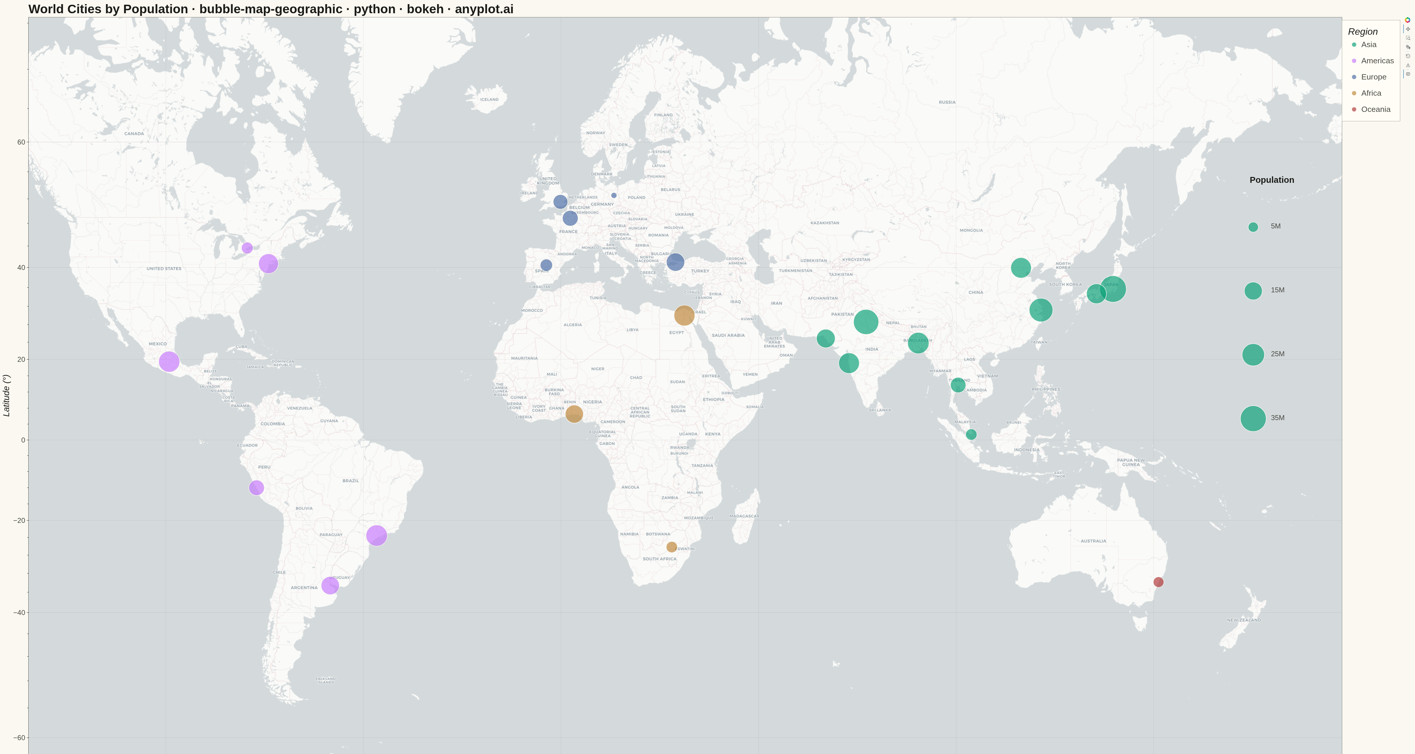
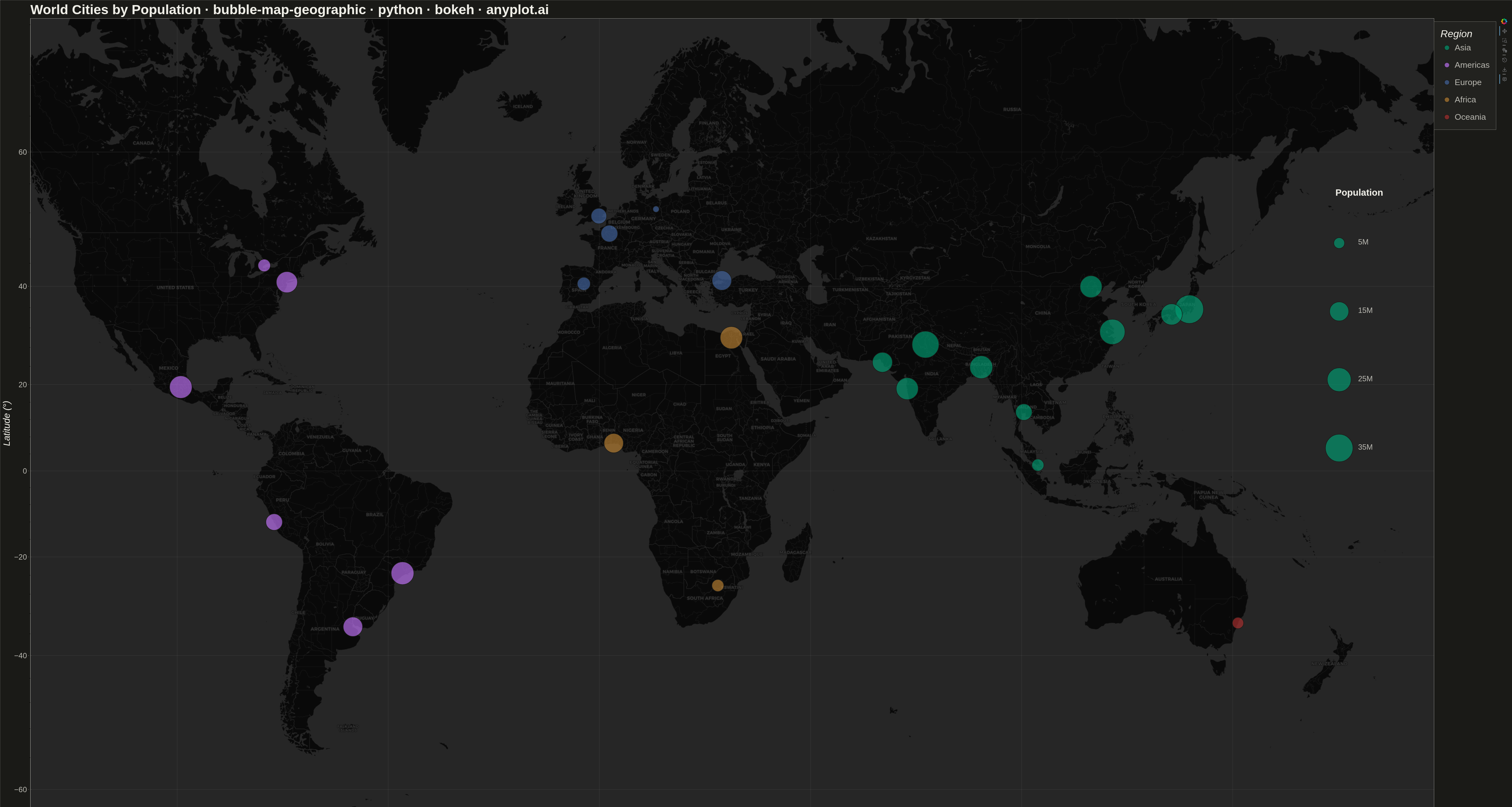
A geographic bubble map where markers are sized proportionally to quantitative data values at each location. Unlike scatter maps where size is optional, bubble maps use marker size as the primary visual encoding to show data magnitude across geographic regions. This visualization makes it immediately apparent where high and low values occur spatially, enabling intuitive comparison of quantities across locations.
""" anyplot.ai
bubble-map-geographic: Bubble Map with Sized Geographic Markers
Library: bokeh 3.9.0 | Python 3.13.13
Quality: 90/100 | Updated: 2026-05-18
"""

import sys


# Remove script directory from sys.path to avoid shadowing the installed bokeh package
# (script is named bokeh.py, which would otherwise shadow the bokeh package on import)
if sys.path and sys.path[0] not in ("", "-c"):
    sys.path.pop(0)

import os
import time
from pathlib import Path

import numpy as np
from bokeh.io import output_file, save
from bokeh.models import ColumnDataSource, LabelSet, Legend, LegendItem, WMTSTileSource
from bokeh.plotting import figure
from bokeh.resources import CDN
from selenium import webdriver
from selenium.webdriver.chrome.options import Options


# Theme tokens
THEME = os.getenv("ANYPLOT_THEME", "light")
PAGE_BG = "#FAF8F1" if THEME == "light" else "#1A1A17"
ELEVATED_BG = "#FFFDF6" if THEME == "light" else "#242420"
INK = "#1A1A17" if THEME == "light" else "#F0EFE8"
INK_SOFT = "#4A4A44" if THEME == "light" else "#B8B7B0"

# Okabe-Ito palette (canonical order)
OKABE = ["#009E73", "#C475FD", "#4467A3", "#BD8233", "#AE3030"]

# Data - World cities with population (in millions, 2024 estimates)
cities = {
    "name": [
        "Tokyo",
        "Delhi",
        "Shanghai",
        "São Paulo",
        "Mexico City",
        "Cairo",
        "Mumbai",
        "Beijing",
        "Dhaka",
        "Osaka",
        "New York",
        "Karachi",
        "Buenos Aires",
        "Istanbul",
        "Lagos",
        "London",
        "Paris",
        "Bangkok",
        "Lima",
        "Sydney",
        "Toronto",
        "Singapore",
        "Berlin",
        "Madrid",
        "Johannesburg",
    ],
    "lat": [
        35.68,
        28.61,
        31.23,
        -23.55,
        19.43,
        30.04,
        19.08,
        39.90,
        23.81,
        34.69,
        40.71,
        24.86,
        -34.60,
        41.01,
        6.52,
        51.51,
        48.86,
        13.76,
        -12.05,
        -33.87,
        43.65,
        1.35,
        52.52,
        40.42,
        -26.20,
    ],
    "lon": [
        139.69,
        77.21,
        121.47,
        -46.63,
        -99.13,
        31.24,
        72.88,
        116.41,
        90.41,
        135.50,
        -74.01,
        67.01,
        -58.38,
        28.98,
        3.38,
        -0.13,
        2.35,
        100.50,
        -77.03,
        151.21,
        -79.38,
        103.82,
        13.40,
        -3.70,
        28.04,
    ],
    "population": [
        37.4,
        32.9,
        28.5,
        22.4,
        21.8,
        21.3,
        20.7,
        20.5,
        22.5,
        19.1,
        18.9,
        16.5,
        15.5,
        15.6,
        15.4,
        9.5,
        11.1,
        10.7,
        10.9,
        5.3,
        6.2,
        5.9,
        3.6,
        6.7,
        5.8,
    ],
    "region": [
        "Asia",
        "Asia",
        "Asia",
        "Americas",
        "Americas",
        "Africa",
        "Asia",
        "Asia",
        "Asia",
        "Asia",
        "Americas",
        "Asia",
        "Americas",
        "Europe",
        "Africa",
        "Europe",
        "Europe",
        "Asia",
        "Americas",
        "Oceania",
        "Americas",
        "Asia",
        "Europe",
        "Europe",
        "Africa",
    ],
}

# Convert lat/lon to Web Mercator projection (EPSG:3857), inlined
k = 6378137
lats = np.array(cities["lat"])
lons = np.array(cities["lon"])
mercator_x = lons * (k * np.pi / 180.0)
mercator_y = np.log(np.tan((90 + lats) * np.pi / 360.0)) * k

populations = np.array(cities["population"])

# Scale bubble area proportionally to population (sqrt for perceptually accurate encoding)
min_size, max_size = 20, 90
pop_normalized = (populations - populations.min()) / (populations.max() - populations.min())
sizes = min_size + np.sqrt(pop_normalized) * (max_size - min_size)

# Okabe-Ito color by region — Asia first gets brand green #009E73
region_order = ["Asia", "Americas", "Europe", "Africa", "Oceania"]
region_colors = {region: OKABE[i] for i, region in enumerate(region_order)}

# Plot
tile_url = (
    "https://tiles.basemaps.cartocdn.com/light_all/{z}/{x}/{y}.png"
    if THEME == "light"
    else "https://tiles.basemaps.cartocdn.com/dark_all/{z}/{x}/{y}.png"
)

p = figure(
    width=4800,
    height=2700,
    x_axis_type="mercator",
    y_axis_type="mercator",
    title="World Cities by Population · bubble-map-geographic · python · bokeh · anyplot.ai",
    tools="pan,wheel_zoom,box_zoom,reset,hover,save",
    tooltips=[
        ("City", "@name"),
        ("Population", "@population{0.0} million"),
        ("Region", "@region"),
        ("Coordinates", "(@lat{0.00}°, @lon{0.00}°)"),
    ],
)

p.add_tile(WMTSTileSource(url=tile_url))

# Bubbles per region, one renderer each for legend
legend_items = []
for region in region_order:
    color = region_colors[region]
    mask = np.array([r == region for r in cities["region"]])
    if mask.any():
        rsrc = ColumnDataSource(
            data={
                "x": mercator_x[mask],
                "y": mercator_y[mask],
                "size": sizes[mask],
                "name": [cities["name"][i] for i in range(len(cities["name"])) if mask[i]],
                "population": populations[mask],
                "region": [region] * mask.sum(),
            }
        )
        renderer = p.scatter(
            x="x",
            y="y",
            source=rsrc,
            size="size",
            fill_color=color,
            fill_alpha=0.65,
            line_color=PAGE_BG,
            line_width=1.5,
        )
        legend_items.append(LegendItem(label=region, renderers=[renderer]))

# Region legend
legend = Legend(
    items=legend_items,
    title="Region",
    title_text_font_size="24pt",
    title_text_color=INK,
    label_text_font_size="20pt",
    label_text_color=INK_SOFT,
    glyph_height=40,
    glyph_width=40,
    spacing=15,
    padding=20,
    background_fill_alpha=0.90,
    background_fill_color=ELEVATED_BG,
    border_line_color=INK_SOFT,
    border_line_width=1,
)
p.add_layout(legend, "right")

# Size reference legend
ref_pops = [5, 15, 25, 35]
ref_x = 19500000
ref_y0 = 6000000
ref_dy = 1800000

ref_sizes = [
    min_size + np.sqrt((pop - populations.min()) / (populations.max() - populations.min())) * (max_size - min_size)
    for pop in ref_pops
]
ref_source = ColumnDataSource(
    data={
        "x": [ref_x] * len(ref_pops),
        "y": [ref_y0 - i * ref_dy for i in range(len(ref_pops))],
        "size": ref_sizes,
        "label": [f"{pop}M" for pop in ref_pops],
    }
)
p.scatter(
    x="x",
    y="y",
    source=ref_source,
    size="size",
    fill_color=OKABE[0],
    fill_alpha=0.65,
    line_color=PAGE_BG,
    line_width=1.5,
)
p.add_layout(
    LabelSet(
        x="x",
        y="y",
        text="label",
        source=ref_source,
        x_offset=60,
        y_offset=-10,
        text_font_size="18pt",
        text_color=INK_SOFT,
        text_align="left",
    )
)
p.text(
    x=[ref_x - 100000],
    y=[ref_y0 + 1200000],
    text=["Population"],
    text_font_size="22pt",
    text_font_style="bold",
    text_color=INK,
)

# Style
p.title.text_font_size = "32pt"
p.title.text_color = INK
p.title.text_font_style = "bold"

p.xaxis.axis_label = "Longitude (°)"
p.yaxis.axis_label = "Latitude (°)"
p.xaxis.axis_label_text_font_size = "22pt"
p.yaxis.axis_label_text_font_size = "22pt"
p.xaxis.axis_label_text_color = INK
p.yaxis.axis_label_text_color = INK
p.xaxis.major_label_text_font_size = "18pt"
p.yaxis.major_label_text_font_size = "18pt"
p.xaxis.major_label_text_color = INK_SOFT
p.yaxis.major_label_text_color = INK_SOFT
p.xaxis.axis_line_color = INK_SOFT
p.yaxis.axis_line_color = INK_SOFT
p.xaxis.major_tick_line_color = INK_SOFT
p.yaxis.major_tick_line_color = INK_SOFT

p.xgrid.grid_line_color = INK
p.ygrid.grid_line_color = INK
p.xgrid.grid_line_alpha = 0.10
p.ygrid.grid_line_alpha = 0.10

p.x_range.start = -15000000
p.x_range.end = 22000000
p.y_range.start = -6000000
p.y_range.end = 8500000

p.background_fill_color = PAGE_BG
p.border_fill_color = PAGE_BG
p.outline_line_color = INK_SOFT

# Save
output_file(f"plot-{THEME}.html")
save(p, title="World Cities by Population · bubble-map-geographic · python · bokeh · anyplot.ai", resources=CDN)

W, H = 4800, 2700
opts = Options()
for arg in (
    "--headless=new",
    "--no-sandbox",
    "--disable-dev-shm-usage",
    "--disable-gpu",
    f"--window-size={W},{H}",
    "--hide-scrollbars",
):
    opts.add_argument(arg)
driver = webdriver.Chrome(options=opts)
driver.set_window_size(W, H)
driver.get(f"file://{Path(f'plot-{THEME}.html').resolve()}")
time.sleep(5)
driver.save_screenshot(f"plot-{THEME}.png")
driver.quit()
Runnable source as JSON, for any HTTP client: https://api.anyplot.ai/specs/bubble-map-geographic/bokeh/code. Any spec id and library id listed in llms-full.txt fit the same URL shape; every URL below is complete and callable.
{
  "spec_id": "bubble-map-geographic",
  "language": "python",
  "library": "bokeh",
  "page": "https://anyplot.ai/bubble-map-geographic/python/bokeh",
  "hub": "https://anyplot.ai/bubble-map-geographic",
  "code_json": "https://api.anyplot.ai/specs/bubble-map-geographic/bokeh/code",
  "spec_json": "https://api.anyplot.ai/specs/bubble-map-geographic",
  "render_light_png": "https://storage.googleapis.com/anyplot-images/plots/bubble-map-geographic/python/bokeh/plot-light.png",
  "render_dark_png": "https://storage.googleapis.com/anyplot-images/plots/bubble-map-geographic/python/bokeh/plot-dark.png",
  "interactive_light_html": "https://storage.googleapis.com/anyplot-images/plots/bubble-map-geographic/python/bokeh/plot-light.html",
  "interactive_dark_html": "https://storage.googleapis.com/anyplot-images/plots/bubble-map-geographic/python/bokeh/plot-dark.html",
  "quality_score": 90.0,
  "license": "MIT",
  "guide": "https://anyplot.ai/llms.txt"
}
Part of Bubble Map with Sized Geographic Markers on anyplot.ai.