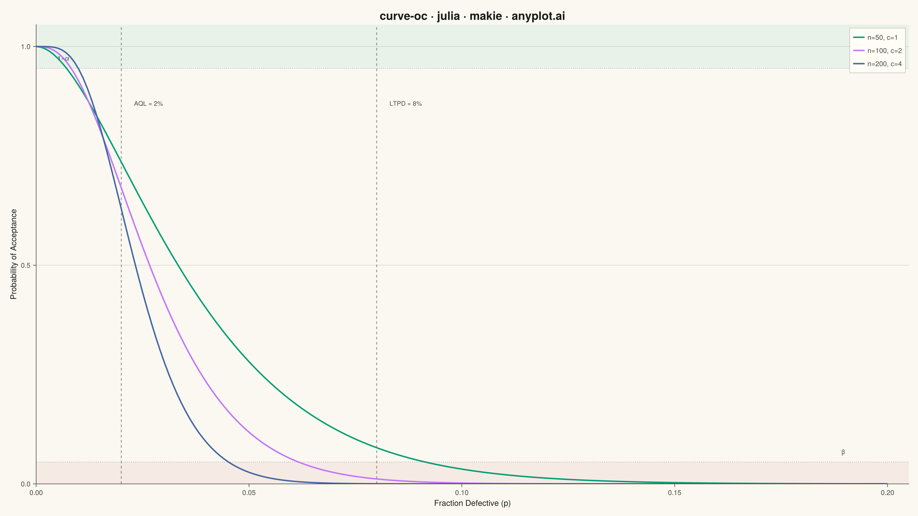
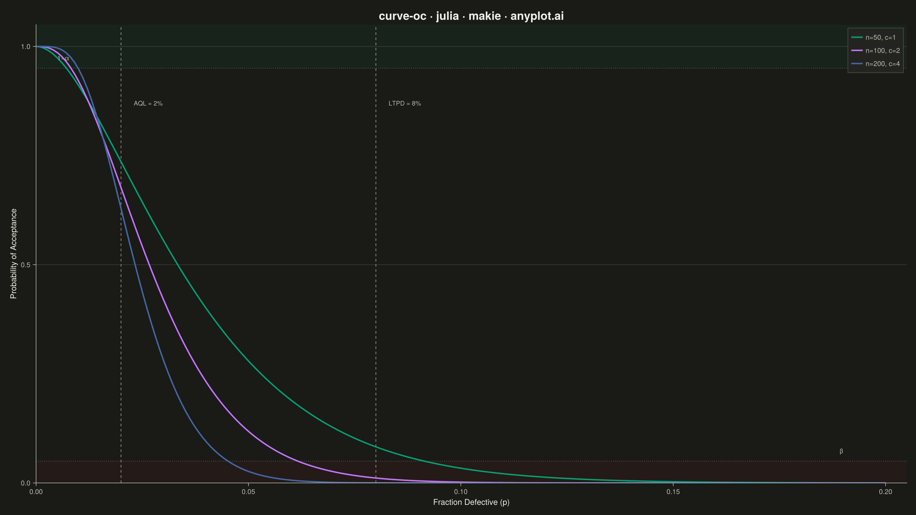
An Operating Characteristic (OC) curve shows the probability of accepting a lot as a function of the true fraction defective in that lot. It is the primary tool for evaluating and comparing acceptance sampling plans, revealing how well an inspection plan discriminates between good and bad lots. The S-shaped curve highlights producer's risk (rejecting good lots) and consumer's risk (accepting bad lots), making it essential for designing effective quality inspection strategies.
# anyplot.ai
# curve-oc: Operating Characteristic (OC) Curve
# Library: makie 0.22.10 | Julia 1.11.9
# Quality: 89/100 | Created: 2026-06-20

using CairoMakie
using Colors
using Random

Random.seed!(42)

# Theme tokens (Imprint palette — theme-adaptive chrome)
const THEME       = get(ENV, "ANYPLOT_THEME", "light")
const PAGE_BG     = THEME == "light" ? colorant"#FAF8F1" : colorant"#1A1A17"
const ELEVATED_BG = THEME == "light" ? colorant"#FFFDF6" : colorant"#242420"
const INK         = THEME == "light" ? colorant"#1A1A17" : colorant"#F0EFE8"
const INK_SOFT    = THEME == "light" ? colorant"#4A4A44" : colorant"#B8B7B0"

const IMPRINT_PALETTE = [
    colorant"#009E73",  # 1 — brand green (always first series)
    colorant"#C475FD",  # 2 — lavender
    colorant"#4467A3",  # 3 — blue
]

# Data — compute OC curves via binomial CDF: P(accept) = sum_{k=0}^{c} C(n,k) p^k (1-p)^(n-k)
oc_prob(n, c, p) = sum(binomial(n, k) * p^k * (1.0 - p)^(n - k) for k in 0:c)
oc_curve(n, c, ps) = [oc_prob(n, c, p) for p in ps]

p_range   = collect(range(0.0, 0.20; length = 200))
plans     = [(50, 1), (100, 2), (200, 4)]
plan_labs = ["n=50, c=1", "n=100, c=2", "n=200, c=4"]
pa_data   = [oc_curve(n, c, p_range) for (n, c) in plans]

aql  = 0.02   # Acceptable Quality Level
ltpd = 0.08   # Lot Tolerance Percent Defective

# Plot
fig = Figure(
    size            = (1600, 900),
    fontsize        = 14,
    backgroundcolor = PAGE_BG,
)

ax = Axis(
    fig[1, 1];
    title             = "curve-oc · julia · makie · anyplot.ai",
    titlesize         = 20,
    titlecolor        = INK,
    xlabel            = "Fraction Defective (p)",
    ylabel            = "Probability of Acceptance",
    xlabelsize        = 14,
    ylabelsize        = 14,
    xlabelcolor       = INK,
    ylabelcolor       = INK,
    xticklabelsize    = 12,
    yticklabelsize    = 12,
    xticklabelcolor   = INK_SOFT,
    yticklabelcolor   = INK_SOFT,
    xtickcolor        = INK_SOFT,
    ytickcolor        = INK_SOFT,
    backgroundcolor   = PAGE_BG,
    topspinevisible   = false,
    rightspinevisible = false,
    leftspinecolor    = INK_SOFT,
    bottomspinecolor  = INK_SOFT,
    xgridvisible      = false,
    ygridcolor        = RGBAf(INK.r, INK.g, INK.b, 0.15),
    xminorgridvisible = false,
    yminorgridvisible = false,
    limits            = (0.0, 0.205, 0.0, 1.05),
)

# Risk zone shading — drawn first so OC curves render on top
hspan!(ax, 0.95, 1.05; color = RGBAf(0.0, 0.62, 0.45, 0.07))   # producer risk (1−α region), brand green tint
hspan!(ax, 0.0,  0.05; color = RGBAf(0.68, 0.19, 0.19, 0.07))  # consumer risk (β region), matte red tint

# AQL and LTPD vertical reference lines
ref_color = RGBAf(INK.r, INK.g, INK.b, 0.45)
vlines!(ax, [aql];  color = ref_color, linestyle = :dash, linewidth = 1.5)
vlines!(ax, [ltpd]; color = ref_color, linestyle = :dash, linewidth = 1.5)

# Producer risk (α) and consumer risk (β) horizontal reference lines
hlines!(ax, [0.95]; color = RGBAf(INK.r, INK.g, INK.b, 0.30), linestyle = :dot, linewidth = 1.2)
hlines!(ax, [0.05]; color = RGBAf(INK.r, INK.g, INK.b, 0.30), linestyle = :dot, linewidth = 1.2)

# OC curves
for (i, (pa, lab)) in enumerate(zip(pa_data, plan_labs))
    lines!(ax, p_range, pa;
           color     = IMPRINT_PALETTE[i],
           linewidth = 2.5,
           label     = lab)
end

# AQL / LTPD labels — raised to y=0.87 to anchor near the high-probability zone
text!(ax, aql + 0.003, 0.87;  text = "AQL = 2%",  color = INK_SOFT, fontsize = 11, align = (:left, :center))
text!(ax, ltpd + 0.003, 0.87; text = "LTPD = 8%", color = INK_SOFT, fontsize = 11, align = (:left, :center))

# Risk threshold labels — 1−α placed on left to avoid legend overlap; β given left padding
text!(ax, 0.005, 0.965; text = "1−α", color = INK_SOFT, fontsize = 11, align = (:left, :bottom))
text!(ax, 0.190, 0.065; text = "β",   color = INK_SOFT, fontsize = 11, align = (:right, :bottom))

axislegend(ax;
           position        = :rt,
           backgroundcolor = ELEVATED_BG,
           labelcolor      = INK_SOFT,
           framecolor      = RGBAf(INK_SOFT.r, INK_SOFT.g, INK_SOFT.b, 0.3),
           labelsize       = 12)

# Save
save("plot-$(THEME).png", fig; px_per_unit = 2)
Runnable source as JSON, for any HTTP client: https://api.anyplot.ai/specs/curve-oc/makie/code. Any spec id and library id listed in llms-full.txt fit the same URL shape; every URL below is complete and callable.
{
  "spec_id": "curve-oc",
  "language": "julia",
  "library": "makie",
  "page": "https://anyplot.ai/curve-oc/julia/makie",
  "hub": "https://anyplot.ai/curve-oc",
  "code_json": "https://api.anyplot.ai/specs/curve-oc/makie/code",
  "spec_json": "https://api.anyplot.ai/specs/curve-oc",
  "render_light_png": "https://storage.googleapis.com/anyplot-images/plots/curve-oc/julia/makie/plot-light.png",
  "render_dark_png": "https://storage.googleapis.com/anyplot-images/plots/curve-oc/julia/makie/plot-dark.png",
  "quality_score": 89.0,
  "license": "MIT",
  "guide": "https://anyplot.ai/llms.txt"
}
Part of Operating Characteristic (OC) Curve on anyplot.ai.