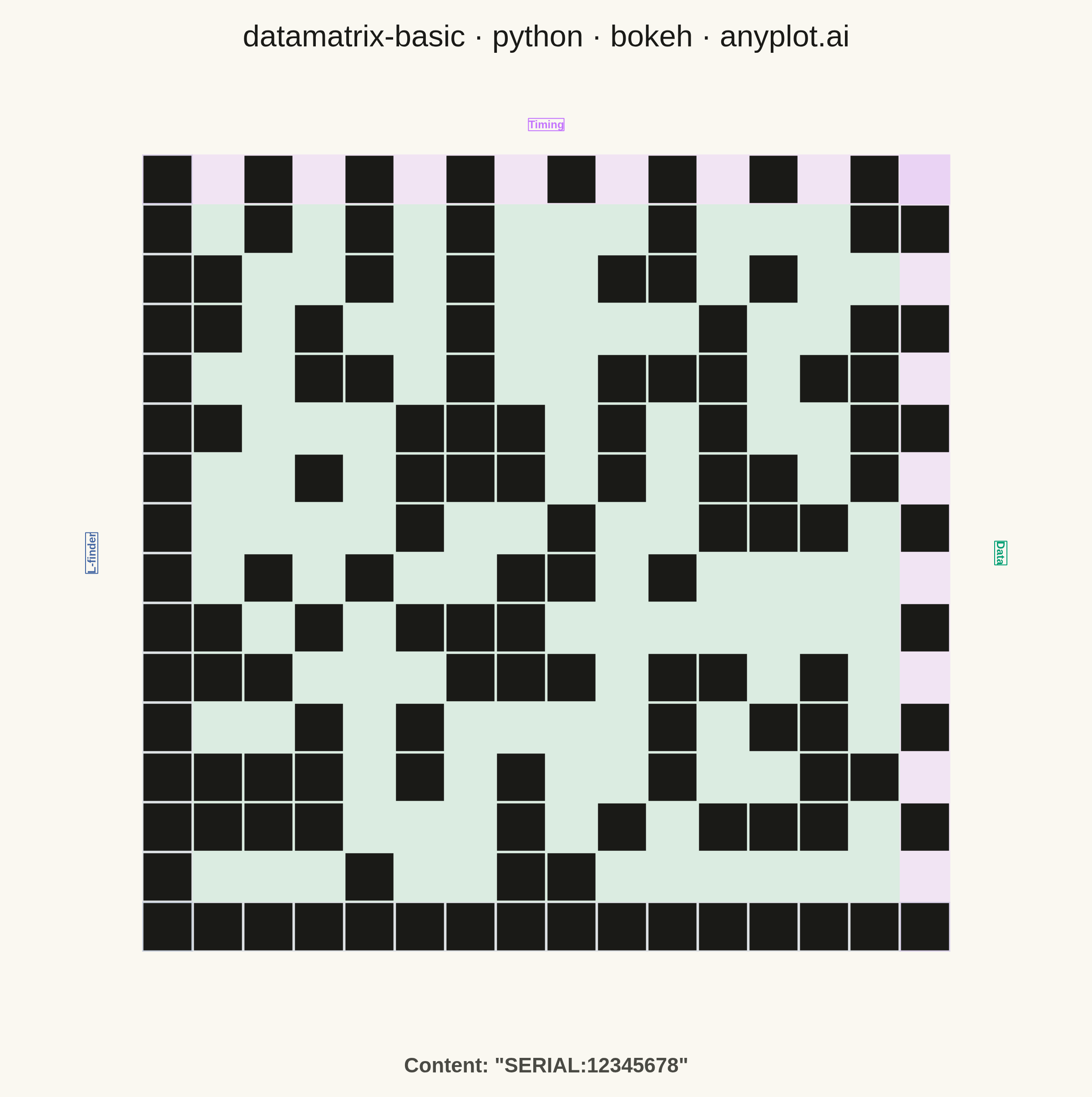
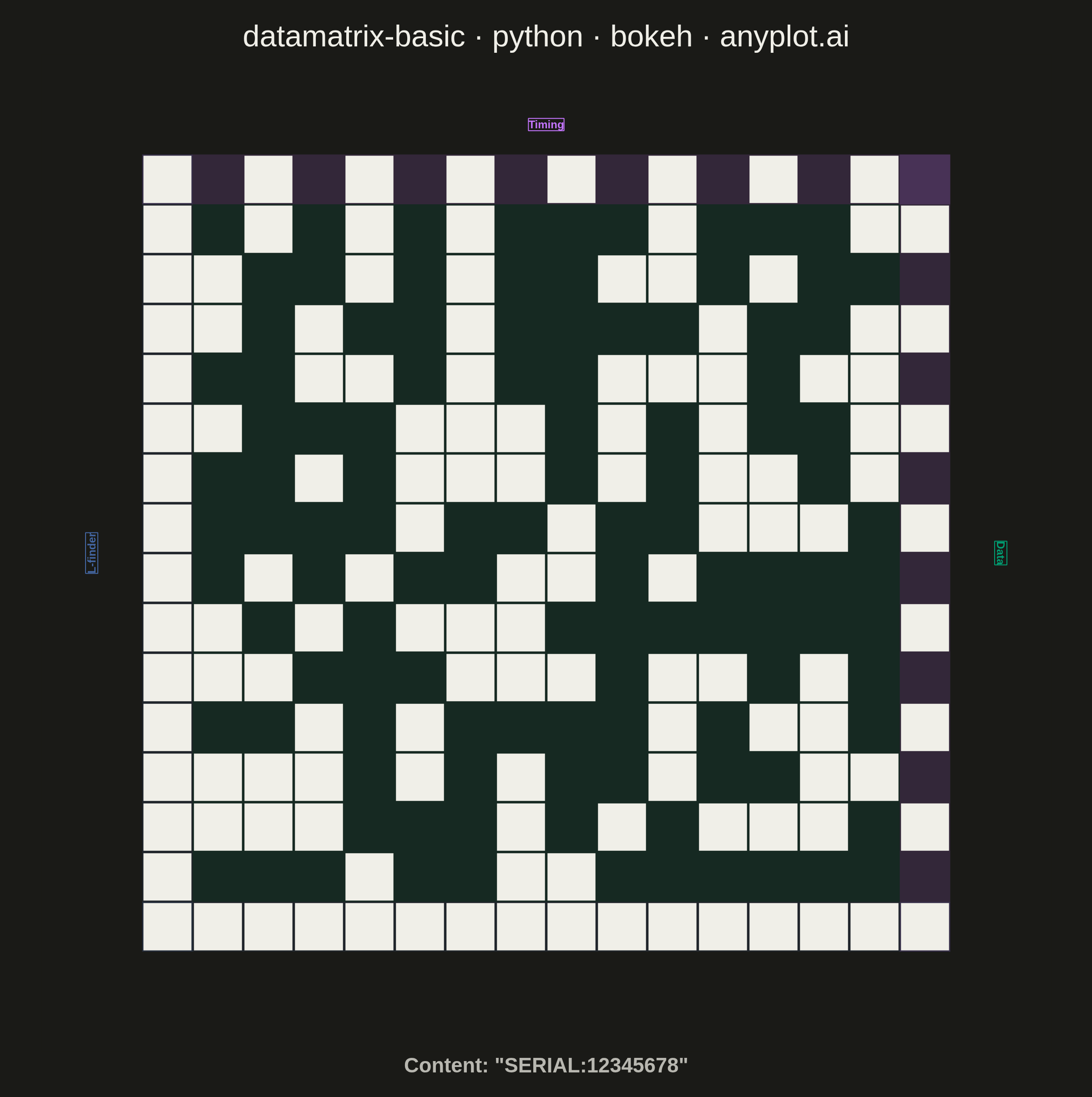
A Data Matrix 2D barcode visualization that encodes data into a compact square or rectangular matrix of black and white cells. Data Matrix codes follow the ISO/IEC 16022 standard, featuring an L-shaped finder pattern (solid borders on two adjacent sides) and alternating timing patterns on the opposite sides. This barcode format is ideal for marking small items and supports high data density with built-in error correction (ECC 200).
""" anyplot.ai
datamatrix-basic: Basic Data Matrix 2D Barcode
Library: bokeh 3.9.0 | Python 3.13.13
Quality: 89/100 | Updated: 2026-05-20
"""

import sys


sys.path.pop(0)  # prevent this file from shadowing the installed bokeh package

import os
import time
from pathlib import Path

import numpy as np
from bokeh.io import output_file, save
from bokeh.models import ColumnDataSource, HoverTool, Label, Title
from bokeh.plotting import figure
from selenium import webdriver
from selenium.webdriver.chrome.options import Options


# Theme tokens
THEME = os.getenv("ANYPLOT_THEME", "light")
PAGE_BG = "#FAF8F1" if THEME == "light" else "#1A1A17"
INK = "#1A1A17" if THEME == "light" else "#F0EFE8"
INK_SOFT = "#4A4A44" if THEME == "light" else "#B8B7B0"

# Data — ASCII-encode "SERIAL:12345678" for a Data Matrix ECC 200 barcode
content = "SERIAL:12345678"

codewords = []
pos_idx = 0
while pos_idx < len(content):
    ch_val = ord(content[pos_idx])
    if pos_idx + 1 < len(content) and content[pos_idx].isdigit() and content[pos_idx + 1].isdigit():
        codewords.append(130 + int(content[pos_idx : pos_idx + 2]))
        pos_idx += 2
    elif 0 <= ch_val <= 127:
        codewords.append(ch_val + 1)
        pos_idx += 1
    else:
        codewords.append(235)
        codewords.append(ch_val - 127)
        pos_idx += 1

# Determine symbol size (capacity, rows, cols) for ECC 200
symbol_sizes = [
    (3, 10, 10),
    (5, 12, 12),
    (8, 14, 14),
    (12, 16, 16),
    (18, 18, 18),
    (22, 20, 20),
    (30, 22, 22),
    (36, 24, 24),
    (44, 26, 26),
]
rows, cols, capacity = 26, 26, 44
for cap, nr, nc in symbol_sizes:
    if len(codewords) <= cap:
        rows, cols, capacity = nr, nc, cap
        break

# Pad codewords to symbol capacity with randomised pad codewords
while len(codewords) < capacity:
    pad_pos = len(codewords) + 1
    pad_cw = 129 + ((149 * pad_pos) % 253) + 1
    if pad_cw > 254:
        pad_cw -= 254
    codewords.append(pad_cw)

# Reed-Solomon ECC — GF(256) with primitive polynomial x^8+x^5+x^3+x^2+1 (=0x12D)
ecc_sizes = {
    (10, 10): 5,
    (12, 12): 7,
    (14, 14): 10,
    (16, 16): 12,
    (18, 18): 14,
    (20, 20): 18,
    (22, 22): 20,
    (24, 24): 24,
    (26, 26): 28,
}
n_ecc = ecc_sizes.get((rows, cols), 10)

gf_prim = 0x12D
gf_exp = [0] * 512
gf_log = [0] * 256
gf_x = 1
for gf_i in range(255):
    gf_exp[gf_i] = gf_x
    gf_log[gf_x] = gf_i
    gf_x <<= 1
    if gf_x >= 256:
        gf_x ^= gf_prim
for gf_i in range(255, 512):
    gf_exp[gf_i] = gf_exp[gf_i - 255]

# Build RS generator polynomial: g(x) = prod(x + alpha^i) for i=0..n_ecc-1
rs_gen = [1]
for ecc_i in range(n_ecc):
    ei = gf_exp[ecc_i]
    new_g = [0] * (len(rs_gen) + 1)
    for g_j, gv in enumerate(rs_gen):
        new_g[g_j] ^= gv
        if gv != 0:
            new_g[g_j + 1] ^= gf_exp[(gf_log[gv] + gf_log[ei]) % 255]
    rs_gen = new_g

# Polynomial long division to compute ECC codewords
rs_rem = list(codewords) + [0] * n_ecc
for d_i in range(len(codewords)):
    coef = rs_rem[d_i]
    if coef != 0:
        for enc_j in range(1, len(rs_gen)):
            if rs_gen[enc_j] != 0:
                rs_rem[d_i + enc_j] ^= gf_exp[(gf_log[rs_gen[enc_j]] + gf_log[coef]) % 255]
all_codewords = codewords + rs_rem[len(codewords) :]

# Construct Data Matrix grid (1=white/light module, 0=dark module)
matrix = np.ones((rows, cols), dtype=int)
matrix[:, 0] = 0  # L-shaped finder: solid left column
matrix[-1, :] = 0  # L-shaped finder: solid bottom row
for ti in range(cols):
    matrix[0, ti] = ti % 2  # Alternating timing on top edge
for ti in range(rows):
    matrix[ti, -1] = (ti + 1) % 2  # Alternating timing on right edge

# Place data bits into inner region, row by row
bit_idx = 0
n_bits = len(all_codewords) * 8
for dr in range(1, rows - 1):
    for dc in range(1, cols - 1):
        if bit_idx < n_bits:
            cw_pos = bit_idx // 8
            bit_pos = 7 - (bit_idx % 8)
            bit_val = (all_codewords[cw_pos] >> bit_pos) & 1
            matrix[dr, dc] = 1 - bit_val  # dark module = 0
            bit_idx += 1

# Compute cell coordinates with quiet zone (2 modules on each side)
quiet = 2
total_w = cols + 2 * quiet
total_h = rows + 2 * quiet
black_rows, black_cols = np.where(matrix == 0)
cell_x = (black_cols + quiet + 0.5).astype(float)
cell_y = (total_h - 1 - (black_rows + quiet) + 0.5).astype(float)
module_types = [
    "L-finder" if (c == 0 or r == rows - 1) else "Timing" if (r == 0 or c == cols - 1) else "Data"
    for r, c in zip(black_rows.tolist(), black_cols.tolist(), strict=True)
]
source = ColumnDataSource(
    data={
        "x": cell_x,
        "y": cell_y,
        "module_row": black_rows.astype(int),
        "module_col": black_cols.astype(int),
        "module_type": module_types,
    }
)

# Plot — 2400×2400 square canvas suits the square Data Matrix barcode
p = figure(
    width=2400,
    height=2400,
    title="datamatrix-basic · python · bokeh · anyplot.ai",
    x_range=(0, total_w),
    y_range=(0, total_h),
    toolbar_location=None,
    min_border_top=120,
    min_border_bottom=90,
    min_border_left=90,
    min_border_right=90,
)

OKABE_BLUE = "#4467A3"
OKABE_ORANGE = "#C475FD"
OKABE_GREEN = "#009E73"

# Structural zone overlays — drawn first so barcode modules render on top
bx = quiet  # barcode left edge in plot coords
by = total_h - quiet - rows  # barcode bottom edge in plot coords
# L-finder: solid left column + solid bottom row
p.rect(x=bx + 0.5, y=by + rows / 2, width=1, height=rows, fill_color=OKABE_BLUE, fill_alpha=0.15, line_color=None)
p.rect(x=bx + cols / 2, y=by + 0.5, width=cols, height=1, fill_color=OKABE_BLUE, fill_alpha=0.15, line_color=None)
# Timing: alternating top row + right column
p.rect(
    x=bx + cols / 2, y=by + rows - 0.5, width=cols, height=1, fill_color=OKABE_ORANGE, fill_alpha=0.15, line_color=None
)
p.rect(
    x=bx + cols - 0.5, y=by + rows / 2, width=1, height=rows, fill_color=OKABE_ORANGE, fill_alpha=0.15, line_color=None
)
# Data region: inner cells (rows 1..rows-2, cols 1..cols-2)
p.rect(
    x=bx + cols / 2,
    y=by + rows / 2,
    width=cols - 2,
    height=rows - 2,
    fill_color=OKABE_GREEN,
    fill_alpha=0.12,
    line_color=None,
)

modules_renderer = p.rect(x="x", y="y", width=0.95, height=0.95, source=source, fill_color=INK, line_color=None)
hover = HoverTool(
    renderers=[modules_renderer], tooltips=[("Type", "@module_type"), ("Row", "@module_row"), ("Col", "@module_col")]
)
p.add_tools(hover)

# Theme-adaptive chrome
p.background_fill_color = PAGE_BG
p.border_fill_color = PAGE_BG
p.outline_line_color = None

p.xaxis.visible = False
p.yaxis.visible = False
p.xgrid.visible = False
p.ygrid.visible = False

p.title.text_font_size = "50pt"
p.title.text_color = INK
p.title.align = "center"
p.title.text_font_style = "normal"

subtitle = Title(text=f'Content: "{content}"', text_font_size="34pt", text_color=INK_SOFT, align="center")
p.add_layout(subtitle, "below")

# Zone labels in the quiet border areas, color-matched to their overlays
for lx, ly, ltxt, lcolor, langle in [
    (1.0, total_h - quiet - rows / 2, "L-finder", OKABE_BLUE, np.pi / 2),
    (quiet + cols / 2, total_h - quiet + 0.6, "Timing", OKABE_ORANGE, 0.0),
    (total_w - 1.0, total_h - quiet - rows / 2, "Data", OKABE_GREEN, -np.pi / 2),
]:
    p.add_layout(
        Label(
            x=lx,
            y=ly,
            text=ltxt,
            text_color=lcolor,
            text_font_size="18pt",
            text_font_style="bold",
            text_align="center",
            text_baseline="middle",
            angle=langle,
            background_fill_color=PAGE_BG,
            background_fill_alpha=0.8,
            border_line_color=lcolor,
            border_line_width=2,
        )
    )

# Save interactive HTML (required catalog artifact)
output_file(f"plot-{THEME}.html")
save(p)

# Screenshot with headless Chrome via Selenium
W, H = 2400, 2400
# Add height buffer to account for headless Chrome's viewport offset (~140px)
WIN_H = H + 150
opts = Options()
for arg in (
    "--headless=new",
    "--no-sandbox",
    "--disable-dev-shm-usage",
    "--disable-gpu",
    f"--window-size={W},{WIN_H}",
    "--hide-scrollbars",
):
    opts.add_argument(arg)
driver = webdriver.Chrome(options=opts)
driver.set_window_size(W, WIN_H)
driver.get(f"file://{Path(f'plot-{THEME}.html').resolve()}")
time.sleep(2)
# Match HTML page background to figure background so no contrast border appears
driver.execute_script(
    "document.body.style.backgroundColor = arguments[0];document.documentElement.style.backgroundColor = arguments[0];",
    PAGE_BG,
)
time.sleep(1)
driver.save_screenshot(f"plot-{THEME}.png")
driver.quit()
Runnable source as JSON, for any HTTP client: https://api.anyplot.ai/specs/datamatrix-basic/bokeh/code. Any spec id and library id listed in llms-full.txt fit the same URL shape; every URL below is complete and callable.
{
  "spec_id": "datamatrix-basic",
  "language": "python",
  "library": "bokeh",
  "page": "https://anyplot.ai/datamatrix-basic/python/bokeh",
  "hub": "https://anyplot.ai/datamatrix-basic",
  "code_json": "https://api.anyplot.ai/specs/datamatrix-basic/bokeh/code",
  "spec_json": "https://api.anyplot.ai/specs/datamatrix-basic",
  "render_light_png": "https://storage.googleapis.com/anyplot-images/plots/datamatrix-basic/python/bokeh/plot-light.png",
  "render_dark_png": "https://storage.googleapis.com/anyplot-images/plots/datamatrix-basic/python/bokeh/plot-dark.png",
  "interactive_light_html": "https://storage.googleapis.com/anyplot-images/plots/datamatrix-basic/python/bokeh/plot-light.html",
  "interactive_dark_html": "https://storage.googleapis.com/anyplot-images/plots/datamatrix-basic/python/bokeh/plot-dark.html",
  "quality_score": 89.0,
  "license": "MIT",
  "guide": "https://anyplot.ai/llms.txt"
}
Part of Basic Data Matrix 2D Barcode on anyplot.ai.