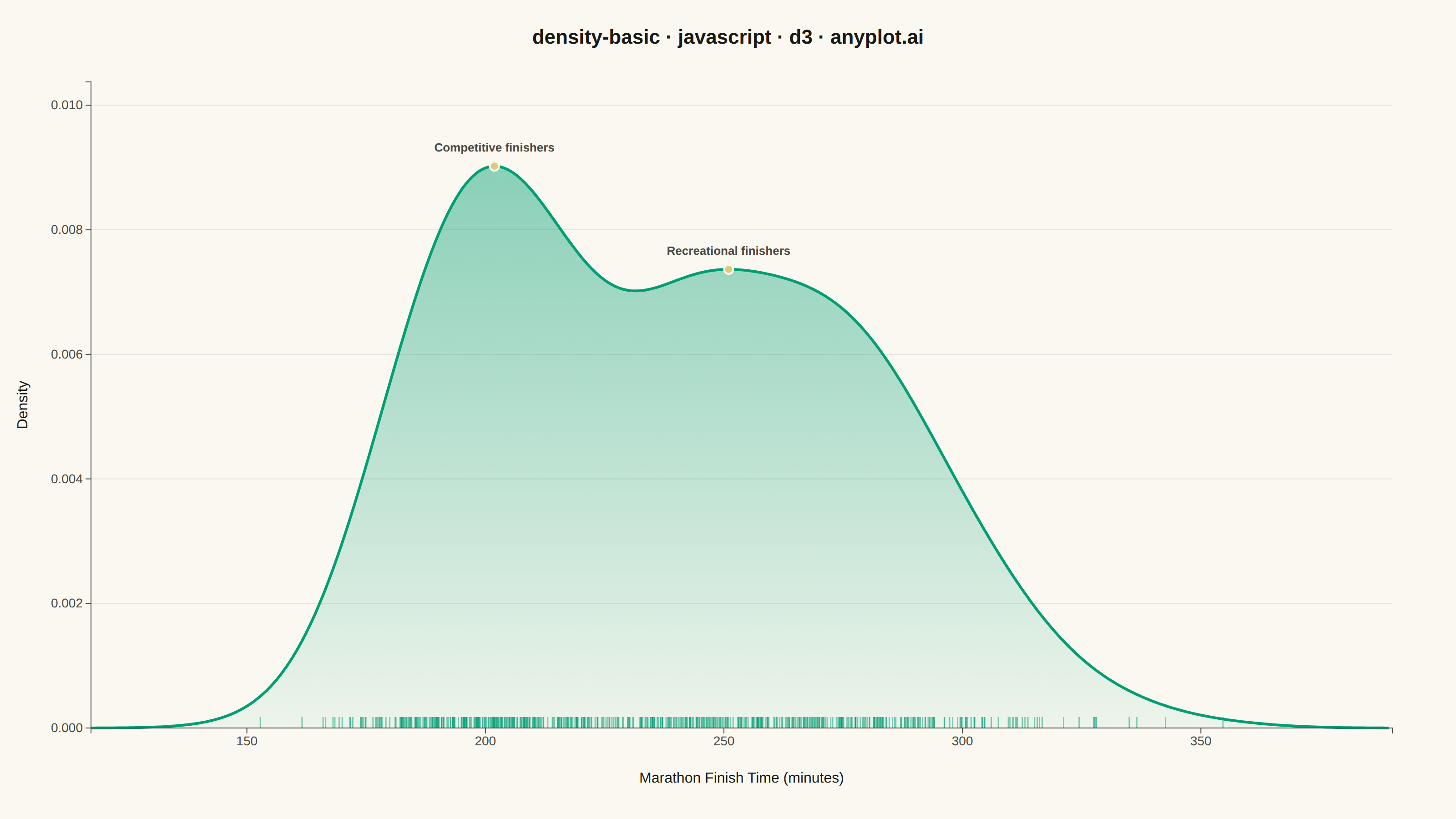
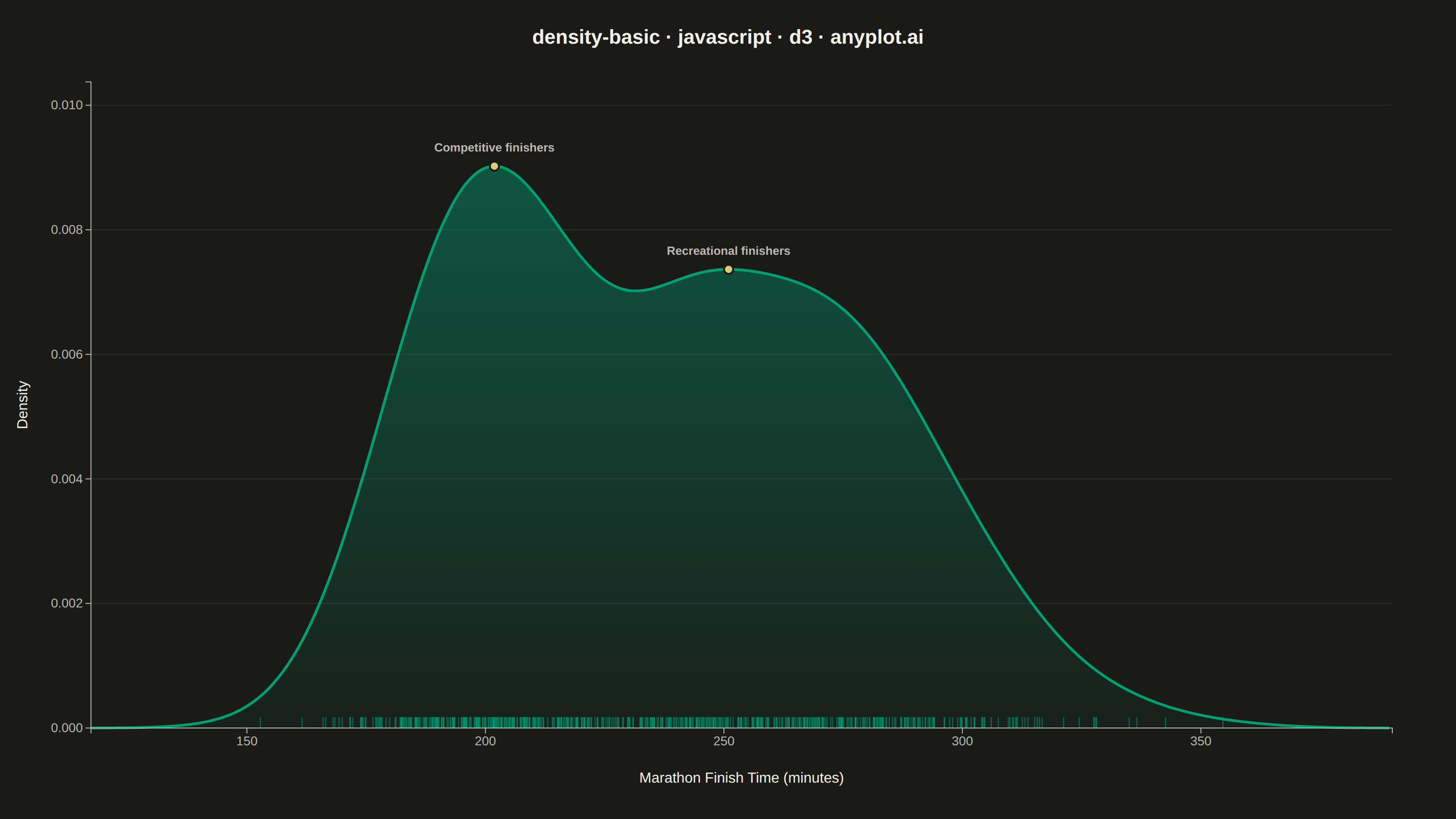
The same plot in 14 other libraries — JavaScript: Chart.js, Apache ECharts, Highcharts, MUI X Charts; Python: Altair, Bokeh, lets-plot, Matplotlib, Plotly, plotnine, Pygal, Seaborn; R: ggplot2; Julia: Makie.jl. Compare all 15 side by side: Basic Density Plot in Python, R, Julia and JavaScript.
A density plot (also known as Kernel Density Estimation or KDE plot) visualizes the distribution of a continuous variable by smoothing the data into a continuous probability density curve. Unlike histograms which use discrete bins, density plots provide a smooth representation of the underlying distribution, making it easier to identify patterns such as skewness, modality, and overall shape.
// anyplot.ai
// density-basic: Basic Density Plot
// Library: d3 7.9.0 | JavaScript 22.23.2
// Quality: 90/100 | Created: 2026-08-24

const t = window.ANYPLOT_TOKENS;
const { width, height } = window.ANYPLOT_SIZE;
const margin = { top: 90, right: 70, bottom: 100, left: 100 };
const iw = width - margin.left - margin.right;
const ih = height - margin.top - margin.bottom;

// --- Data: marathon finish times (minutes), mixture of competitive and
// recreational runners so the density curve shows a subtle bimodal shape ---
function lcg(seed) {
  let state = seed % 2147483647;
  if (state <= 0) state += 2147483646;
  return function () {
    state = (state * 16807) % 2147483647;
    return (state - 1) / 2147483646;
  };
}
const rand = lcg(42);
function randomNormal(mean, sd) {
  const u1 = rand();
  const u2 = rand();
  const z = Math.sqrt(-2 * Math.log(u1)) * Math.cos(2 * Math.PI * u2);
  return mean + z * sd;
}

const finishTimes = [];
for (let i = 0; i < 600; i++) {
  const isCompetitive = rand() < 0.3;
  const time = isCompetitive ? randomNormal(195, 15) : randomNormal(258, 32);
  finishTimes.push(Math.max(120, time));
}

// --- Kernel density estimation (Gaussian kernel, Silverman bandwidth) ------
const meanTime = d3.mean(finishTimes);
const stdTime = d3.deviation(finishTimes);
const bandwidth = 1.06 * stdTime * Math.pow(finishTimes.length, -1 / 5);

function kernelGaussian(bw) {
  return (v) => Math.exp(-0.5 * (v / bw) ** 2) / (bw * Math.sqrt(2 * Math.PI));
}
function kde(kernel, sample, xValues) {
  return xValues.map((x) => [x, d3.mean(sample, (v) => kernel(x - v))]);
}

const domainMin = d3.min(finishTimes) - 3 * bandwidth;
const domainMax = d3.max(finishTimes) + 3 * bandwidth;
const grid = d3.range(domainMin, domainMax, (domainMax - domainMin) / 400);
const density = kde(kernelGaussian(bandwidth), finishTimes, grid);

// --- SVG mount ---------------------------------------------------------------
const svg = d3.select("#container").append("svg").attr("width", width).attr("height", height);
const g = svg.append("g").attr("transform", `translate(${margin.left},${margin.top})`);

// --- Scales -------------------------------------------------------------------
const x = d3.scaleLinear().domain([domainMin, domainMax]).range([0, iw]);
const y = d3
  .scaleLinear()
  .domain([0, d3.max(density, (d) => d[1]) * 1.15])
  .range([ih, 0]);

// --- Y grid (subtle, y-axis only) --------------------------------------------
g.append("g")
  .attr("class", "grid")
  .call(d3.axisLeft(y).ticks(5).tickSize(-iw).tickFormat(""))
  .call((sel) => sel.select(".domain").remove())
  .call((sel) => sel.selectAll("line").attr("stroke", t.grid).attr("stroke-opacity", 0.6));

// --- Area + line --------------------------------------------------------------
// Vertical fill gradient (denser near the curve, fading toward the baseline)
// for more visual depth than a flat fill-opacity.
const gradientId = "density-fill-gradient";
svg
  .append("defs")
  .append("linearGradient")
  .attr("id", gradientId)
  .attr("x1", "0%")
  .attr("y1", "0%")
  .attr("x2", "0%")
  .attr("y2", "100%")
  .call((grad) => {
    grad.append("stop").attr("offset", "0%").attr("stop-color", t.palette[0]).attr("stop-opacity", 0.45);
    grad.append("stop").attr("offset", "100%").attr("stop-color", t.palette[0]).attr("stop-opacity", 0.05);
  });

const area = d3
  .area()
  .x((d) => x(d[0]))
  .y0(ih)
  .y1((d) => y(d[1]));

const line = d3
  .line()
  .x((d) => x(d[0]))
  .y((d) => y(d[1]));

g.append("path").datum(density).attr("d", area).attr("fill", `url(#${gradientId})`);
g.append("path")
  .datum(density)
  .attr("d", line)
  .attr("fill", "none")
  .attr("stroke", t.palette[0])
  .attr("stroke-width", 3);

// --- Rug plot: individual observations along the baseline --------------------
g.append("g")
  .selectAll("line")
  .data(finishTimes)
  .join("line")
  .attr("x1", (d) => x(d))
  .attr("x2", (d) => x(d))
  .attr("y1", ih)
  .attr("y2", ih - 12)
  .attr("stroke", t.palette[0])
  .attr("stroke-width", 1.4)
  .attr("stroke-opacity", 0.5);

// --- Peak annotations: call out the two-population (bimodal) shape ----------
const maxDensity = d3.max(density, (d) => d[1]);
const localMaxima = [];
for (let i = 1; i < density.length - 1; i++) {
  const dCur = density[i][1];
  if (dCur > density[i - 1][1] && dCur > density[i + 1][1] && dCur > maxDensity * 0.3) {
    localMaxima.push(density[i]);
  }
}
const peaks = localMaxima
  .sort((a, b) => b[1] - a[1])
  .slice(0, 2)
  .sort((a, b) => a[0] - b[0]);
const peakLabels = ["Competitive finishers", "Recreational finishers"];

const peakGroup = g.append("g");
peaks.forEach(([px, py], i) => {
  const cx = x(px);
  const cy = y(py);
  peakGroup
    .append("circle")
    .attr("cx", cx)
    .attr("cy", cy)
    .attr("r", 5)
    .attr("fill", t.amber)
    .attr("stroke", t.pageBg)
    .attr("stroke-width", 2);
  if (peakLabels[i]) {
    peakGroup
      .append("text")
      .attr("x", cx)
      .attr("y", cy - 16)
      .attr("text-anchor", "middle")
      .attr("fill", t.inkSoft)
      .style("font-size", "13px")
      .style("font-weight", "600")
      .text(peakLabels[i]);
  }
});

// --- Axes -----------------------------------------------------------------
const xAxis = g
  .append("g")
  .attr("transform", `translate(0,${ih})`)
  .call(d3.axisBottom(x).ticks(8));
const yAxis = g.append("g").call(d3.axisLeft(y).ticks(5).tickFormat(d3.format(".3f")));
for (const axis of [xAxis, yAxis]) {
  axis.selectAll("text").attr("fill", t.inkSoft).style("font-size", "14px");
  axis.selectAll("line").attr("stroke", t.inkSoft);
  axis.select(".domain").attr("stroke", t.inkSoft);
}

// --- Axis labels ---------------------------------------------------------
g.append("text")
  .attr("x", iw / 2)
  .attr("y", ih + 60)
  .attr("text-anchor", "middle")
  .attr("fill", t.ink)
  .style("font-size", "16px")
  .text("Marathon Finish Time (minutes)");

g.append("text")
  .attr("transform", "rotate(-90)")
  .attr("x", -ih / 2)
  .attr("y", -70)
  .attr("text-anchor", "middle")
  .attr("fill", t.ink)
  .style("font-size", "16px")
  .text("Density");

// --- Title ---------------------------------------------------------------
svg
  .append("text")
  .attr("x", width / 2)
  .attr("y", 48)
  .attr("text-anchor", "middle")
  .attr("fill", t.ink)
  .style("font-size", "22px")
  .style("font-weight", "600")
  .text("density-basic · javascript · d3 · anyplot.ai");
Runnable source as JSON, for any HTTP client: https://api.anyplot.ai/specs/density-basic/d3/code. Any spec id and library id listed in llms-full.txt fit the same URL shape; every URL below is complete and callable.
{
  "spec_id": "density-basic",
  "language": "javascript",
  "library": "d3",
  "page": "https://anyplot.ai/density-basic/javascript/d3",
  "hub": "https://anyplot.ai/density-basic",
  "code_json": "https://api.anyplot.ai/specs/density-basic/d3/code",
  "spec_json": "https://api.anyplot.ai/specs/density-basic",
  "render_light_png": "https://storage.googleapis.com/anyplot-images/plots/density-basic/javascript/d3/plot-light.png",
  "render_dark_png": "https://storage.googleapis.com/anyplot-images/plots/density-basic/javascript/d3/plot-dark.png",
  "interactive_light_html": "https://storage.googleapis.com/anyplot-images/plots/density-basic/javascript/d3/plot-light.html",
  "interactive_dark_html": "https://storage.googleapis.com/anyplot-images/plots/density-basic/javascript/d3/plot-dark.html",
  "quality_score": 90.0,
  "license": "MIT",
  "guide": "https://anyplot.ai/llms.txt"
}
Part of Basic Density Plot on anyplot.ai.