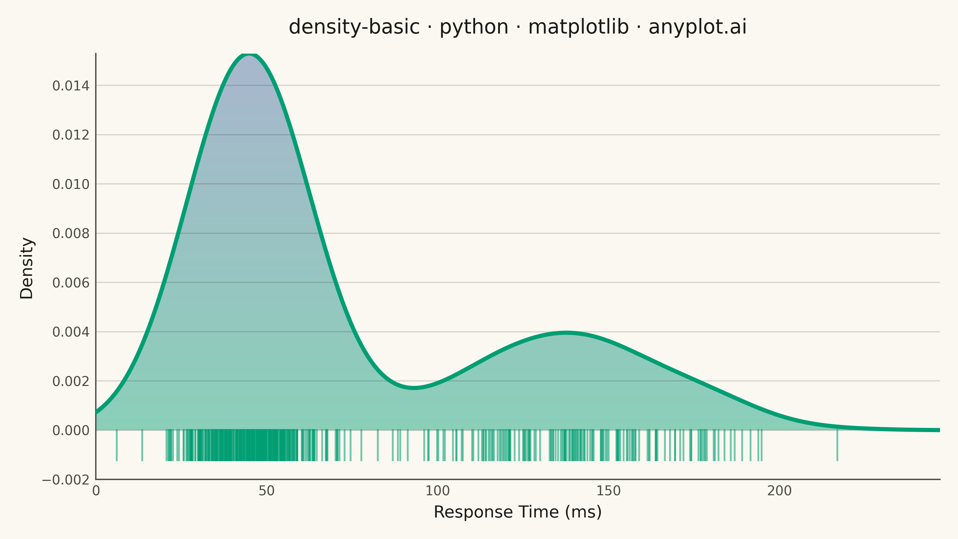
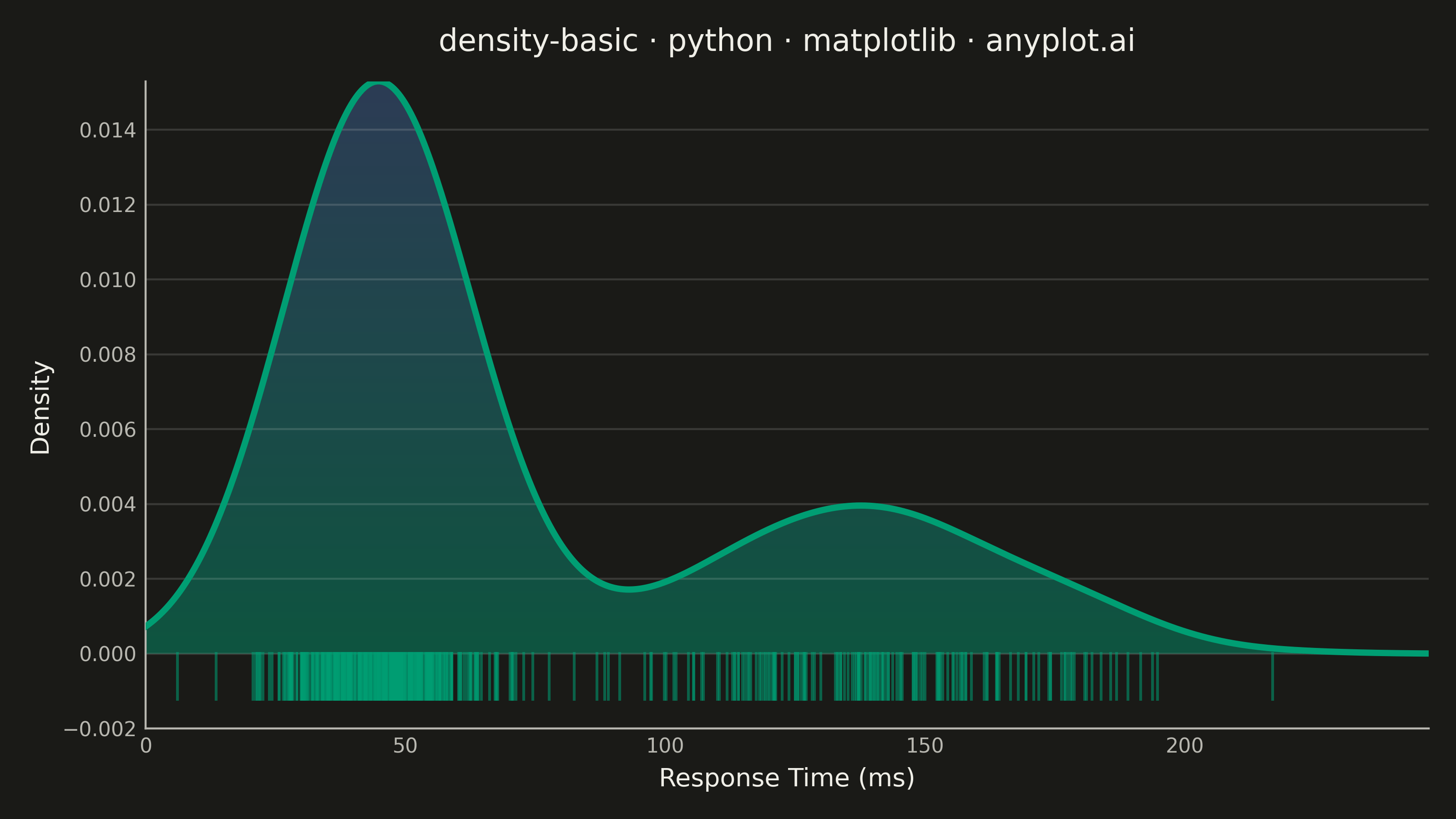
A density plot (also known as Kernel Density Estimation or KDE plot) visualizes the distribution of a continuous variable by smoothing the data into a continuous probability density curve. Unlike histograms which use discrete bins, density plots provide a smooth representation of the underlying distribution, making it easier to identify patterns such as skewness, modality, and overall shape.
""" anyplot.ai
density-basic: Basic Density Plot
Library: matplotlib 3.10.9 | Python 3.13.13
Quality: 89/100 | Updated: 2026-05-30
"""

import os

import matplotlib.pyplot as plt
import matplotlib.ticker as ticker
import numpy as np
from matplotlib.collections import EventCollection
from matplotlib.colors import LinearSegmentedColormap
from matplotlib.patches import PathPatch
from matplotlib.path import Path
from scipy import stats
from scipy.signal import argrelextrema


# Theme tokens
THEME = os.getenv("ANYPLOT_THEME", "light")
PAGE_BG = "#FAF8F1" if THEME == "light" else "#1A1A17"
ELEVATED_BG = "#FFFDF6" if THEME == "light" else "#242420"
INK = "#1A1A17" if THEME == "light" else "#F0EFE8"
INK_SOFT = "#4A4A44" if THEME == "light" else "#B8B7B0"
INK_MUTED = "#6B6A63" if THEME == "light" else "#A8A79F"
BRAND = "#009E73"  # Imprint palette position 1 — ALWAYS first series

# Data - Response times (ms) showing bimodal server behavior
np.random.seed(42)
cached_responses = np.random.normal(45, 12, 350)  # Fast cache-hit requests
db_responses = np.random.normal(140, 25, 150)  # Slower database-query requests
response_times = np.concatenate([cached_responses, db_responses])
response_times = response_times[response_times > 0]

# Compute KDE with Silverman bandwidth selection
kde = stats.gaussian_kde(response_times, bw_method="silverman")
x_range = np.linspace(0, response_times.max() + 30, 600)
density = kde(x_range)

# Plot
fig, ax = plt.subplots(figsize=(8, 4.5), dpi=400, facecolor=PAGE_BG)
ax.set_facecolor(PAGE_BG)

# Imprint sequential gradient fill clipped to density curve via PathPatch
imprint_seq = LinearSegmentedColormap.from_list("imprint_seq", [BRAND, "#4467A3"])
gradient = np.linspace(0, 1, 256).reshape(-1, 1)
ax.imshow(
    gradient,
    extent=[x_range[0], x_range[-1], 0, density.max()],
    aspect="auto",
    cmap=imprint_seq,
    alpha=0.45,
    origin="lower",
    zorder=1,
)
verts = np.column_stack([np.concatenate([x_range, [x_range[-1], x_range[0]]]), np.concatenate([density, [0, 0]])])
codes = [Path.MOVETO] + [Path.LINETO] * (len(verts) - 1)
clip_path = PathPatch(Path(verts, codes), transform=ax.transData, facecolor="none", edgecolor="none")
ax.add_patch(clip_path)
for artist in ax.get_images():
    artist.set_clip_path(clip_path)

# Density curve
ax.plot(x_range, density, linewidth=2.5, color=BRAND, zorder=3)

# Rug plot via EventCollection — slightly more prominent for full-resolution visibility
rug = EventCollection(
    response_times, lineoffset=-0.0006, linelength=0.0013, linewidth=1.1, color=BRAND, alpha=0.55, zorder=2
)
ax.add_collection(rug)

# Style
title = "density-basic · python · matplotlib · anyplot.ai"
title_n = len(title)
title_fontsize = max(8, round(12 * 67 / title_n)) if title_n > 67 else 12

ax.set_xlabel("Response Time (ms)", fontsize=10, color=INK)
ax.set_ylabel("Density", fontsize=10, color=INK)
ax.set_title(title, fontsize=title_fontsize, fontweight="medium", color=INK, pad=12)
ax.tick_params(axis="both", labelsize=8, colors=INK_SOFT, length=0)
ax.xaxis.set_major_formatter(ticker.FormatStrFormatter("%g"))

# Grid and spines
ax.yaxis.grid(True, alpha=0.15, linewidth=0.8, color=INK)
ax.spines["top"].set_visible(False)
ax.spines["right"].set_visible(False)
ax.spines["left"].set_color(INK_SOFT)
ax.spines["bottom"].set_color(INK_SOFT)

# Axis limits — bottom offset accommodates rug plot ticks below zero
ax.set_xlim(x_range[0], x_range[-1])
ax.set_ylim(bottom=-0.0020)

# Suppress the negative y-axis tick label (rug offset lives there, not real density)
ax.yaxis.set_major_formatter(ticker.FuncFormatter(lambda v, _: "" if v < 0 else f"{v:.4g}"))

# Locate the two KDE peaks and annotate them
peak_idxs = argrelextrema(density, np.greater, order=25)[0]
if len(peak_idxs) >= 2:
    p1_idx, p2_idx = peak_idxs[0], peak_idxs[1]
else:
    # Fallback: split range at midpoint and take each half's argmax
    mid = len(x_range) // 2
    p1_idx = np.argmax(density[:mid])
    p2_idx = mid + np.argmax(density[mid:])

p1_x, p1_y = x_range[p1_idx], density[p1_idx]
p2_x, p2_y = x_range[p2_idx], density[p2_idx]

annotation_kw = {
    "fontsize": 8,
    "color": INK_SOFT,
    "bbox": {"facecolor": ELEVATED_BG, "edgecolor": INK_SOFT, "alpha": 0.88, "boxstyle": "round,pad=0.3"},
    "arrowprops": {"arrowstyle": "->", "color": INK_MUTED, "lw": 1.0},
    "ha": "center",
}
ax.annotate(f"Cache hit\n~{p1_x:.0f} ms", xy=(p1_x, p1_y), xytext=(p1_x - 15, p1_y * 0.60), **annotation_kw)
ax.annotate(f"DB query\n~{p2_x:.0f} ms", xy=(p2_x, p2_y), xytext=(p2_x + 22, p2_y * 0.70), **annotation_kw)

plt.tight_layout()

# Save — no bbox_inches='tight' (preserves exact 3200×1800 canvas)
plt.savefig(f"plot-{THEME}.png", dpi=400, facecolor=PAGE_BG)
Runnable source as JSON, for any HTTP client: https://api.anyplot.ai/specs/density-basic/matplotlib/code. Any spec id and library id listed in llms-full.txt fit the same URL shape; every URL below is complete and callable.
{
  "spec_id": "density-basic",
  "language": "python",
  "library": "matplotlib",
  "page": "https://anyplot.ai/density-basic/python/matplotlib",
  "hub": "https://anyplot.ai/density-basic",
  "code_json": "https://api.anyplot.ai/specs/density-basic/matplotlib/code",
  "spec_json": "https://api.anyplot.ai/specs/density-basic",
  "render_light_png": "https://storage.googleapis.com/anyplot-images/plots/density-basic/python/matplotlib/plot-light.png",
  "render_dark_png": "https://storage.googleapis.com/anyplot-images/plots/density-basic/python/matplotlib/plot-dark.png",
  "quality_score": 89.0,
  "license": "MIT",
  "guide": "https://anyplot.ai/llms.txt"
}
Part of Basic Density Plot on anyplot.ai.