The same plot in 14 other libraries — JavaScript: Chart.js, D3.js, Highcharts, MUI X Charts; Python: Altair, Bokeh, lets-plot, Matplotlib, Plotly, plotnine, Pygal, Seaborn; R: ggplot2; Julia: Makie.jl. Compare all 15 side by side: Basic Density Plot in Python, R, Julia and JavaScript.
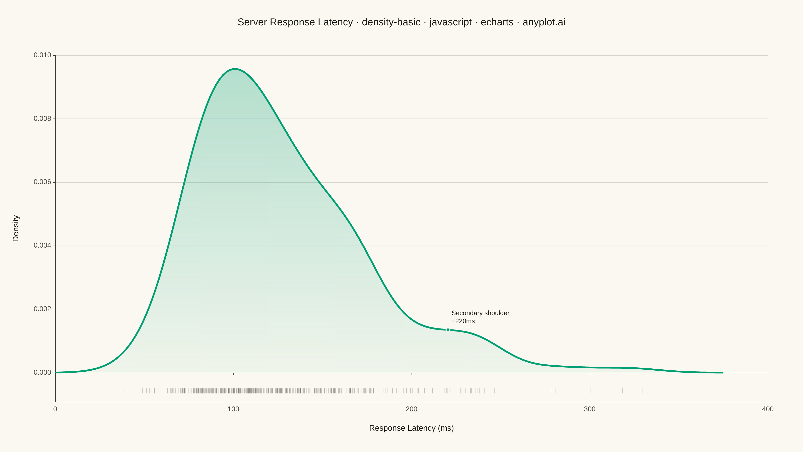
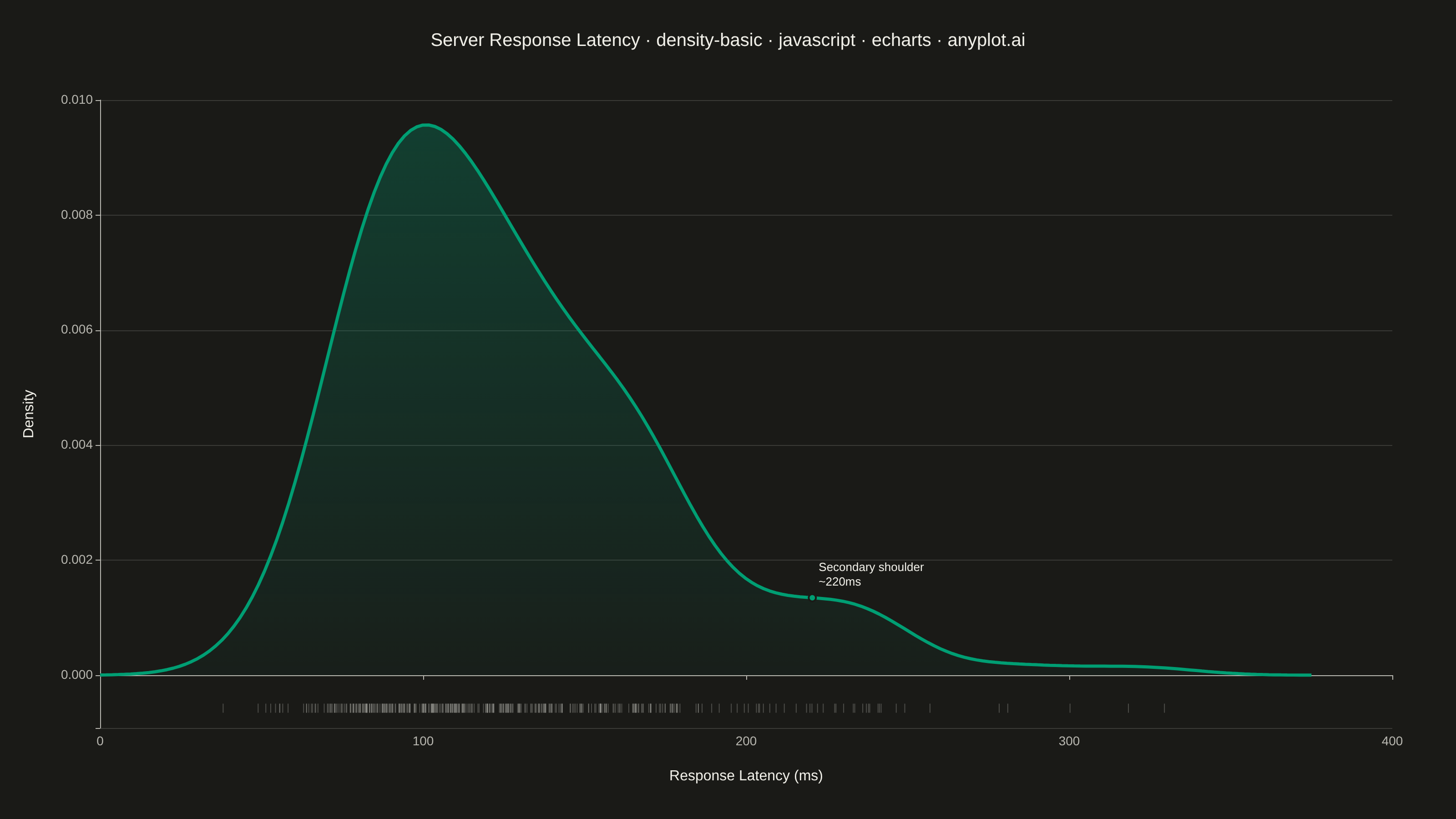
A density plot (also known as Kernel Density Estimation or KDE plot) visualizes the distribution of a continuous variable by smoothing the data into a continuous probability density curve. Unlike histograms which use discrete bins, density plots provide a smooth representation of the underlying distribution, making it easier to identify patterns such as skewness, modality, and overall shape.
// anyplot.ai
// density-basic: Basic Density Plot
// Library: echarts 6.1.0 | JavaScript 22.23.2
// Quality: 91/100 | Created: 2026-08-24

const t = window.ANYPLOT_TOKENS;

// --- Data: server response latency (ms), right-skewed --------------------
function mulberry32(seed) {
  return function () {
    seed |= 0;
    seed = (seed + 0x6d2b79f5) | 0;
    let x = Math.imul(seed ^ (seed >>> 15), 1 | seed);
    x = (x + Math.imul(x ^ (x >>> 7), 61 | x)) ^ x;
    return ((x ^ (x >>> 14)) >>> 0) / 4294967296;
  };
}
const rand = mulberry32(42);

function randNormal() {
  let u = 0;
  let v = 0;
  while (u === 0) u = rand();
  while (v === 0) v = rand();
  return Math.sqrt(-2 * Math.log(u)) * Math.cos(2 * Math.PI * v);
}

const sampleCount = 400;
const logMean = Math.log(120); // median latency ~120ms
const logStd = 0.35;
const latencies = [];
for (let i = 0; i < sampleCount; i++) {
  latencies.push(Math.exp(logMean + logStd * randNormal()));
}

// --- Gaussian KDE with Silverman's rule-of-thumb bandwidth ----------------
const mean = latencies.reduce((a, b) => a + b, 0) / sampleCount;
const variance =
  latencies.reduce((a, b) => a + (b - mean) ** 2, 0) / (sampleCount - 1);
const std = Math.sqrt(variance);
const bandwidth = 1.06 * std * Math.pow(sampleCount, -1 / 5);

function gaussianKernel(u) {
  return Math.exp(-0.5 * u * u) / Math.sqrt(2 * Math.PI);
}

const vmin = Math.min(...latencies);
const vmax = Math.max(...latencies);
const pad = bandwidth * 3;
const gridStart = Math.max(0, vmin - pad);
const gridEnd = vmax + pad;
const gridCount = 200;
const step = (gridEnd - gridStart) / (gridCount - 1);

const densityCurve = [];
let peakDensity = 0;
for (let i = 0; i < gridCount; i++) {
  const x = gridStart + i * step;
  let sum = 0;
  for (let j = 0; j < sampleCount; j++) {
    sum += gaussianKernel((x - latencies[j]) / bandwidth);
  }
  const density = sum / (sampleCount * bandwidth);
  peakDensity = Math.max(peakDensity, density);
  densityCurve.push([x, density]);
}

// Rug plot: individual observations as ticks below the curve
const rugY = -peakDensity * 0.06;
const rugData = latencies.map((v) => [v, rugY]);

// Round the x-axis to clean bounds instead of the raw KDE grid extent
const xMax = Math.ceil(gridEnd / 50) * 50;

// Detect the secondary shoulder in the tail: not a true local maximum (the
// curve keeps descending overall), but a flattening of the descent — a local
// maximum in the curve's slope. Look for the point in the tail (past the
// global peak) where the descent visibly slows before continuing downward.
let globalPeakIdx = 0;
for (let i = 1; i < densityCurve.length; i++) {
  if (densityCurve[i][1] > densityCurve[globalPeakIdx][1]) globalPeakIdx = i;
}
// Widened second derivative (concavity): a shoulder is the point of
// strongest local "bulge" (concave-up interruption of the otherwise
// concave-down decline). A window of several grid steps rides over the
// sample-noise wobble that a point-to-point derivative would chase.
const w = 8;
let bulgeStartIdx = -1;
let bestBulge = 0;
for (let i = globalPeakIdx + w + 2; i < densityCurve.length - w - 2; i++) {
  const bulge =
    densityCurve[i - w][1] - 2 * densityCurve[i][1] + densityCurve[i + w][1];
  if (bulge > bestBulge) {
    bestBulge = bulge;
    bulgeStartIdx = i;
  }
}
// The bulge marks where the descent starts to flatten; walk forward a bit
// further to land the label on the flattest part of the shelf itself.
let shoulderIdx = bulgeStartIdx;
if (bulgeStartIdx >= 0) {
  let flattest = Infinity;
  const scanEnd = Math.min(bulgeStartIdx + 30, densityCurve.length - 2);
  for (let i = bulgeStartIdx; i <= scanEnd; i++) {
    const localSlope = Math.abs(
      densityCurve[i + 1][1] - densityCurve[i - 1][1],
    );
    if (localSlope < flattest) {
      flattest = localSlope;
      shoulderIdx = i;
    }
  }
}
const shoulderPoint = shoulderIdx >= 0 ? densityCurve[shoulderIdx] : null;

// Vertical gradient fill: fuller near the curve, fading toward the baseline.
function hexToRgba(hex, alpha) {
  const n = parseInt(hex.slice(1), 16);
  return `rgba(${(n >> 16) & 255}, ${(n >> 8) & 255}, ${n & 255}, ${alpha})`;
}
const areaGradient = new echarts.graphic.LinearGradient(0, 0, 0, 1, [
  { offset: 0, color: hexToRgba(t.palette[0], 0.4) },
  { offset: 1, color: hexToRgba(t.palette[0], 0.06) },
]);

// --- Init -------------------------------------------------------------------
const chart = echarts.init(document.getElementById("container"));

// --- Option -----------------------------------------------------------------
const title =
  "Server Response Latency · density-basic · javascript · echarts · anyplot.ai";

chart.setOption({
  animation: false,
  color: t.palette,
  backgroundColor: "transparent",
  title: {
    text: title,
    left: "center",
    top: 30,
    textStyle: { color: t.ink, fontSize: 20, fontWeight: 500 },
  },
  grid: { left: 110, right: 70, top: 110, bottom: 100 },
  xAxis: {
    type: "value",
    name: "Response Latency (ms)",
    nameLocation: "middle",
    nameGap: 45,
    nameTextStyle: { color: t.ink, fontSize: 16 },
    min: 0,
    max: xMax,
    axisLabel: { color: t.inkSoft, fontSize: 14 },
    axisLine: { lineStyle: { color: t.inkSoft } },
    splitLine: { show: false },
  },
  yAxis: {
    type: "value",
    name: "Density",
    nameLocation: "middle",
    nameGap: 70,
    nameTextStyle: { color: t.ink, fontSize: 16 },
    min: rugY * 1.6,
    axisLabel: {
      color: t.inkSoft,
      fontSize: 14,
      formatter: (v) => (v < 0 ? "" : v.toFixed(3)),
    },
    axisLine: { lineStyle: { color: t.inkSoft } },
    splitLine: { lineStyle: { color: t.grid } },
  },
  series: [
    {
      name: "Density",
      type: "line",
      data: densityCurve,
      symbol: "none",
      smooth: false,
      lineStyle: { color: t.palette[0], width: 3.5 },
      areaStyle: { color: areaGradient },
      markPoint: shoulderPoint
        ? {
            silent: true,
            symbol: "circle",
            symbolSize: 8,
            itemStyle: {
              color: t.palette[0],
              borderColor: t.pageBg,
              borderWidth: 2,
            },
            label: {
              show: true,
              formatter: `Secondary shoulder\n~${Math.round(shoulderPoint[0])}ms`,
              color: t.ink,
              fontSize: 13,
              fontWeight: 500,
              align: "left",
              position: [12, -36],
              lineHeight: 16,
            },
            data: [{ coord: shoulderPoint, name: "shoulder" }],
          }
        : undefined,
      z: 2,
    },
    {
      name: "Observations",
      type: "scatter",
      data: rugData,
      symbol: "rect",
      symbolSize: [1, 10],
      itemStyle: { color: t.inkSoft, opacity: 0.32 },
      z: 1,
    },
  ],
});
Runnable source as JSON, for any HTTP client: https://api.anyplot.ai/specs/density-basic/echarts/code. Any spec id and library id listed in llms-full.txt fit the same URL shape; every URL below is complete and callable.
{
  "spec_id": "density-basic",
  "language": "javascript",
  "library": "echarts",
  "page": "https://anyplot.ai/density-basic/javascript/echarts",
  "hub": "https://anyplot.ai/density-basic",
  "code_json": "https://api.anyplot.ai/specs/density-basic/echarts/code",
  "spec_json": "https://api.anyplot.ai/specs/density-basic",
  "render_light_png": "https://storage.googleapis.com/anyplot-images/plots/density-basic/javascript/echarts/plot-light.png",
  "render_dark_png": "https://storage.googleapis.com/anyplot-images/plots/density-basic/javascript/echarts/plot-dark.png",
  "interactive_light_html": "https://storage.googleapis.com/anyplot-images/plots/density-basic/javascript/echarts/plot-light.html",
  "interactive_dark_html": "https://storage.googleapis.com/anyplot-images/plots/density-basic/javascript/echarts/plot-dark.html",
  "quality_score": 91.0,
  "license": "MIT",
  "guide": "https://anyplot.ai/llms.txt"
}
Part of Basic Density Plot on anyplot.ai.