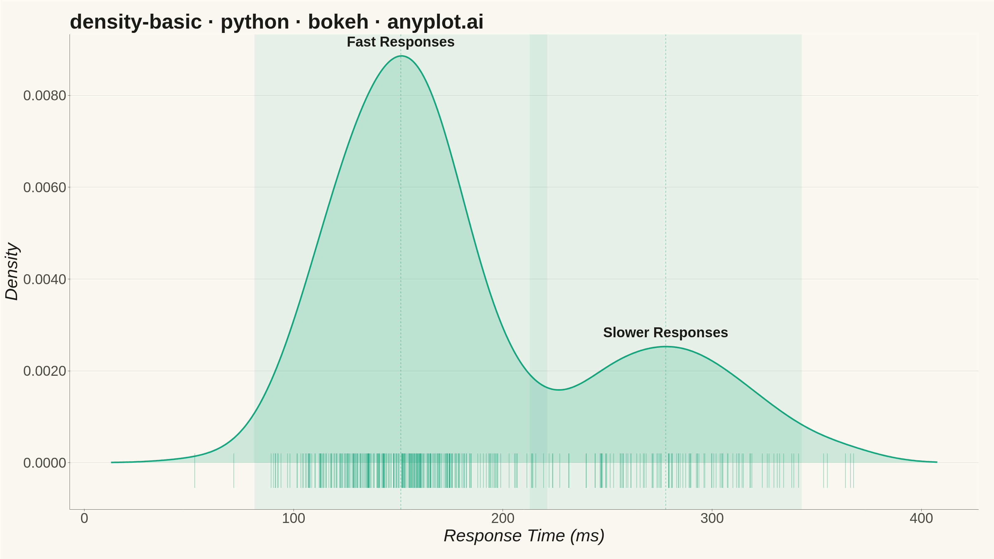
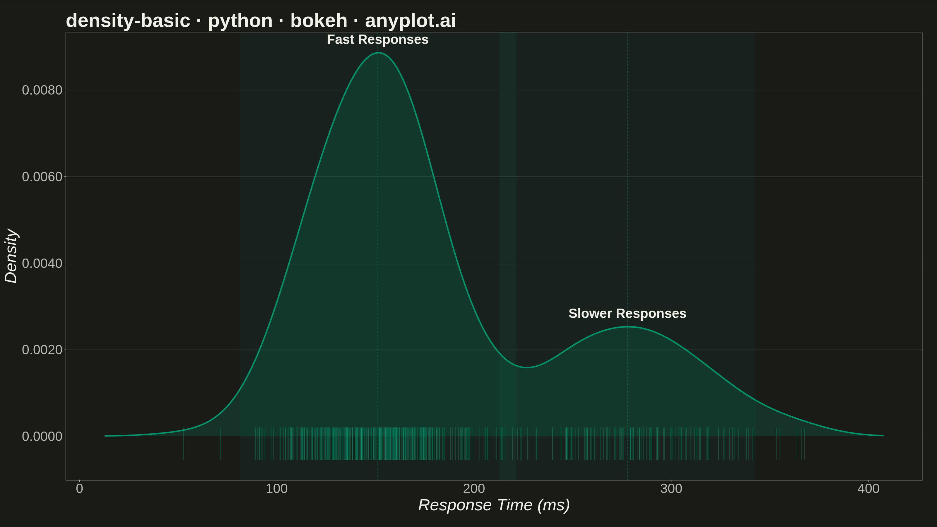
A density plot (also known as Kernel Density Estimation or KDE plot) visualizes the distribution of a continuous variable by smoothing the data into a continuous probability density curve. Unlike histograms which use discrete bins, density plots provide a smooth representation of the underlying distribution, making it easier to identify patterns such as skewness, modality, and overall shape.
""" anyplot.ai
density-basic: Basic Density Plot
Library: bokeh 3.9.0 | Python 3.13.13
Quality: 91/100 | Updated: 2026-05-30
"""

import os
import sys


# This file is named bokeh.py — remove its directory from sys.path so imports
# resolve to the installed bokeh package rather than this script itself.
_script_dir = os.path.dirname(os.path.abspath(__file__))
sys.path = [p for p in sys.path if os.path.abspath(p) != _script_dir]

import time
from pathlib import Path

import numpy as np
from bokeh.io import output_file, save
from bokeh.models import BoxAnnotation, ColumnDataSource, HoverTool, Label, NumeralTickFormatter, Span
from bokeh.plotting import figure
from selenium import webdriver
from selenium.webdriver.chrome.options import Options


THEME = os.getenv("ANYPLOT_THEME", "light")

# Imprint palette — theme-adaptive chrome
PAGE_BG = "#FAF8F1" if THEME == "light" else "#1A1A17"
ELEVATED_BG = "#FFFDF6" if THEME == "light" else "#242420"
INK = "#1A1A17" if THEME == "light" else "#F0EFE8"
INK_SOFT = "#4A4A44" if THEME == "light" else "#B8B7B0"
INK_MUTED = "#6B6A63" if THEME == "light" else "#A8A79F"

# Imprint palette — first categorical series is always #009E73
BRAND = "#009E73"

# Data — response times (ms) for a web service showing bimodal distribution
np.random.seed(42)
response_times = np.concatenate(
    [
        np.random.normal(150, 30, 300),  # Fast responses
        np.random.normal(280, 40, 100),  # Slower responses (bimodal tail)
    ]
)

# Kernel density estimation — Silverman's rule for bandwidth
n = len(response_times)
std = np.std(response_times)
iqr = np.percentile(response_times, 75) - np.percentile(response_times, 25)
bandwidth = 0.9 * min(std, iqr / 1.34) * n ** (-0.2)

# Evaluate KDE on a fine grid
x_grid = np.linspace(response_times.min() - 40, response_times.max() + 40, 500)
density = np.zeros_like(x_grid)
for xi in response_times:
    density += np.exp(-0.5 * ((x_grid - xi) / bandwidth) ** 2)
density /= n * bandwidth * np.sqrt(2 * np.pi)

# Locate the two mode peaks for data storytelling
peak1_idx = np.argmax(density[:250])
peak2_idx = 250 + np.argmax(density[250:])
peak1_x, peak1_y = x_grid[peak1_idx], density[peak1_idx]
peak2_x, peak2_y = x_grid[peak2_idx], density[peak2_idx]

# ColumnDataSource for density curve (enables HoverTool)
source = ColumnDataSource(data={"x": x_grid, "density": density})

# Rug plot — individual observations as vertical segments at y=0
rug_y0 = -0.00055
rug_y1 = rug_y0 + 0.00075
rug_source = ColumnDataSource(
    data={"x": response_times, "y0": np.full_like(response_times, rug_y0), "y1": np.full_like(response_times, rug_y1)}
)

# Figure — canonical 3200×1800 landscape canvas
p = figure(
    width=3200,
    height=1800,
    title="density-basic · python · bokeh · anyplot.ai",
    x_axis_label="Response Time (ms)",
    y_axis_label="Density",
    toolbar_location=None,
    min_border_bottom=160,
    min_border_left=180,
    min_border_top=110,
    min_border_right=50,
)

# BoxAnnotation highlights each modal region — idiomatic Bokeh way to shade bands
box1 = BoxAnnotation(left=peak1_x - 70, right=peak1_x + 70, fill_color=BRAND, fill_alpha=0.07, line_color=None)
box2 = BoxAnnotation(left=peak2_x - 65, right=peak2_x + 65, fill_color=BRAND, fill_alpha=0.07, line_color=None)
p.add_layout(box1)
p.add_layout(box2)

# Span — vertical dashed reference lines at each peak (Bokeh-idiomatic)
for px in (peak1_x, peak2_x):
    p.add_layout(
        Span(location=px, dimension="height", line_color=BRAND, line_width=2, line_dash="dashed", line_alpha=0.45)
    )

# Fill under the density curve
p.varea(x="x", y1=0, y2="density", source=source, fill_color=BRAND, fill_alpha=0.18)

# Density curve (primary glyph; also the HoverTool target)
density_line = p.line(x="x", y="density", source=source, line_color=BRAND, line_width=5, line_alpha=0.9)

# Peak annotations
for px, py, label in ((peak1_x, peak1_y, "Fast Responses"), (peak2_x, peak2_y, "Slower Responses")):
    p.add_layout(
        Label(
            x=px,
            y=py,
            text=label,
            text_font_size="34pt",
            text_color=INK,
            text_font_style="bold",
            text_align="center",
            y_offset=20,
        )
    )

# HoverTool — vline mode follows cursor along the curve
hover = HoverTool(
    renderers=[density_line],
    tooltips=[("Response Time", "@x{0.0} ms"), ("Density", "@density{0.00000}")],
    mode="vline",
    line_policy="nearest",
)
p.add_tools(hover)

# Rug plot — reduced alpha to ease visual crowding in the primary cluster
p.segment(x0="x", y0="y0", x1="x", y1="y1", source=rug_source, line_color=BRAND, line_width=2, line_alpha=0.38)

# Text sizing — canonical native-pixel values for 3200×1800
p.title.text_font_size = "50pt"
p.title.text_color = INK
p.xaxis.axis_label_text_font_size = "42pt"
p.yaxis.axis_label_text_font_size = "42pt"
p.xaxis.major_label_text_font_size = "34pt"
p.yaxis.major_label_text_font_size = "34pt"
p.xaxis.axis_label_text_color = INK
p.yaxis.axis_label_text_color = INK
p.xaxis.major_label_text_color = INK_SOFT
p.yaxis.major_label_text_color = INK_SOFT

# Y-axis numeric format
p.yaxis.formatter = NumeralTickFormatter(format="0.0000")

# Axis chrome — theme-adaptive
p.xaxis.axis_line_color = INK_SOFT
p.yaxis.axis_line_color = INK_SOFT
p.xaxis.axis_line_width = 1
p.yaxis.axis_line_width = 1
p.xaxis.minor_tick_line_color = None
p.yaxis.minor_tick_line_color = None
p.xaxis.major_tick_line_color = INK_SOFT
p.yaxis.major_tick_line_color = INK_SOFT

# Grid — y-axis only, subtle
p.xgrid.grid_line_color = None
p.ygrid.grid_line_color = INK
p.ygrid.grid_line_alpha = 0.15
p.ygrid.grid_line_width = 1

# Background and border
p.background_fill_color = PAGE_BG
p.border_fill_color = PAGE_BG
p.outline_line_color = None

# Save interactive HTML (required catalog artifact)
output_file(f"plot-{THEME}.html")
save(p)

# Screenshot with headless Chrome — Selenium 4 / Selenium Manager
W, H = 3200, 1800
opts = Options()
for arg in (
    "--headless=new",
    "--no-sandbox",
    "--disable-dev-shm-usage",
    "--disable-gpu",
    f"--window-size={W},{H}",
    "--hide-scrollbars",
):
    opts.add_argument(arg)
driver = webdriver.Chrome(options=opts)
# CDP override is authoritative — --window-size alone loses ~139 px to Chrome chrome
driver.execute_cdp_cmd(
    "Emulation.setDeviceMetricsOverride", {"width": W, "height": H, "deviceScaleFactor": 1, "mobile": False}
)
driver.get(f"file://{Path(f'plot-{THEME}.html').resolve()}")
time.sleep(3)
driver.save_screenshot(f"plot-{THEME}.png")
driver.quit()

# Normalize to exact 3200×1800 — guards against ±1–2 px rounding in headless Chrome
from PIL import Image as _Image


_img = _Image.open(f"plot-{THEME}.png")
if _img.size != (W, H):
    _norm = _Image.new("RGB", (W, H), PAGE_BG)
    _norm.paste(_img, ((W - _img.size[0]) // 2, (H - _img.size[1]) // 2))
    _norm.save(f"plot-{THEME}.png")
Runnable source as JSON, for any HTTP client: https://api.anyplot.ai/specs/density-basic/bokeh/code. Any spec id and library id listed in llms-full.txt fit the same URL shape; every URL below is complete and callable.
{
  "spec_id": "density-basic",
  "language": "python",
  "library": "bokeh",
  "page": "https://anyplot.ai/density-basic/python/bokeh",
  "hub": "https://anyplot.ai/density-basic",
  "code_json": "https://api.anyplot.ai/specs/density-basic/bokeh/code",
  "spec_json": "https://api.anyplot.ai/specs/density-basic",
  "render_light_png": "https://storage.googleapis.com/anyplot-images/plots/density-basic/python/bokeh/plot-light.png",
  "render_dark_png": "https://storage.googleapis.com/anyplot-images/plots/density-basic/python/bokeh/plot-dark.png",
  "interactive_light_html": "https://storage.googleapis.com/anyplot-images/plots/density-basic/python/bokeh/plot-light.html",
  "interactive_dark_html": "https://storage.googleapis.com/anyplot-images/plots/density-basic/python/bokeh/plot-dark.html",
  "quality_score": 91.0,
  "license": "MIT",
  "guide": "https://anyplot.ai/llms.txt"
}
Part of Basic Density Plot on anyplot.ai.