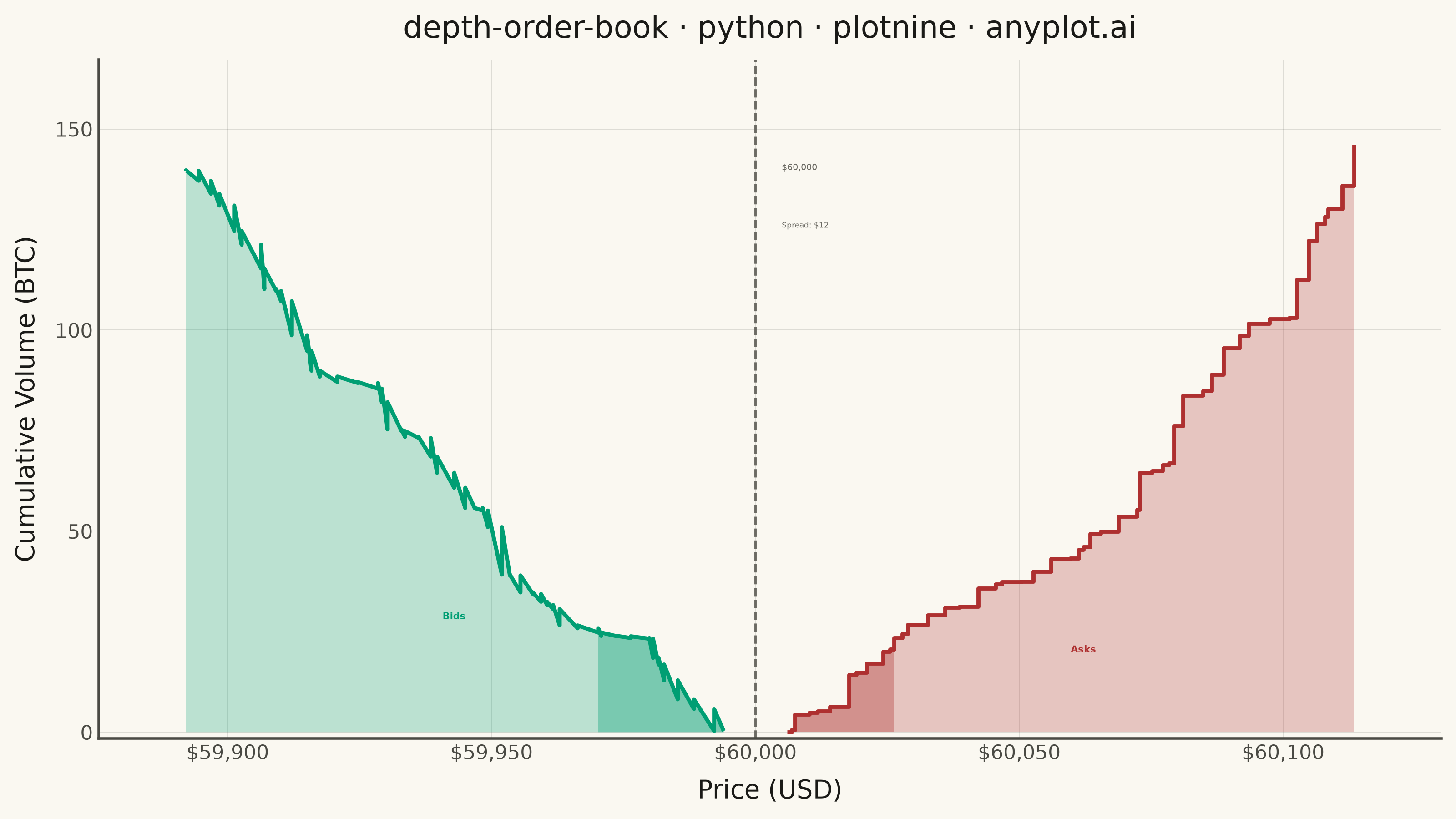
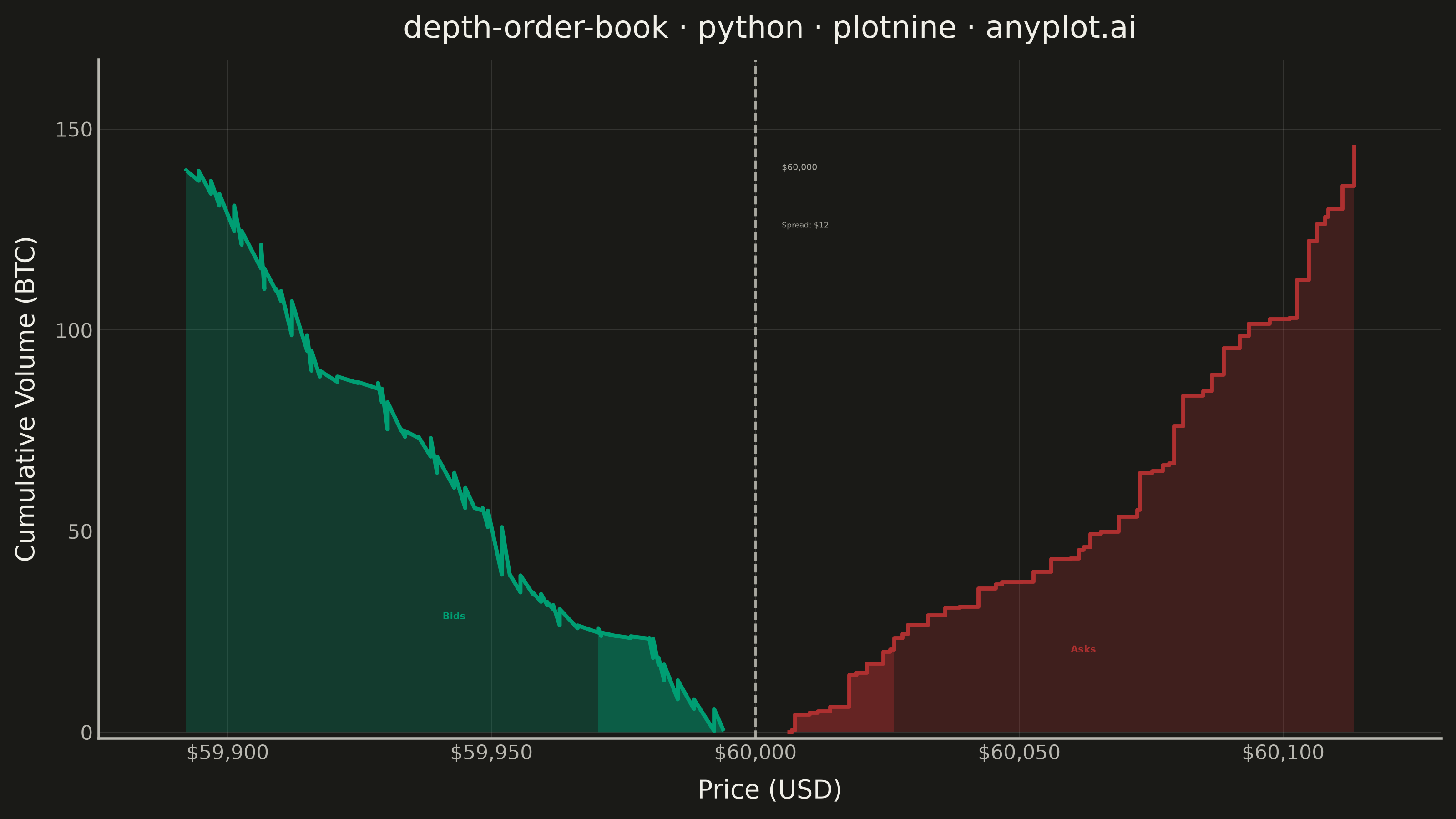
A market depth chart visualizes a snapshot of an exchange order book as two cumulative step areas around the mid price. Cumulative bid volume rises as a green step area to the left of the mid price (summing buy orders from the best bid downward), while cumulative ask volume rises as a red step area to the right (summing sell orders from the best ask upward). The bid-ask spread appears as a gap at the center, with price on the x-axis and cumulative quantity on the y-axis. This is the iconic chart found in nearly every trading and crypto exchange UI, revealing liquidity, support/resistance walls, and the imbalance between buying and selling pressure.
""" anyplot.ai
depth-order-book: Order Book Depth Chart
Library: plotnine 0.15.7 | Python 3.13.13
Quality: 88/100 | Created: 2026-06-15
"""

import os
import sys


sys.path = [p for p in sys.path if os.path.abspath(p) != os.getcwd()]

import numpy as np
import pandas as pd
from plotnine import (
    aes,
    annotate,
    coord_cartesian,
    element_blank,
    element_line,
    element_rect,
    element_text,
    geom_line,
    geom_ribbon,
    geom_vline,
    ggplot,
    labs,
    scale_x_continuous,
    scale_y_continuous,
    theme,
    theme_minimal,
)


# Theme tokens
THEME = os.getenv("ANYPLOT_THEME", "light")
PAGE_BG = "#FAF8F1" if THEME == "light" else "#1A1A17"
ELEVATED_BG = "#FFFDF6" if THEME == "light" else "#242420"
INK = "#1A1A17" if THEME == "light" else "#F0EFE8"
INK_SOFT = "#4A4A44" if THEME == "light" else "#B8B7B0"
INK_MUTED = "#6B6A63" if THEME == "light" else "#A8A79F"

# Imprint palette — semantic: green=bids (buy), red=asks (sell)
BID_COLOR = "#009E73"  # Imprint position 1 — first series; green for bid/buy pressure
ASK_COLOR = "#AE3030"  # Imprint position 5 — semantic anchor for loss/sell pressure

# Data — synthetic BTC/USD order book snapshot
np.random.seed(42)
mid_price = 60_000.0
spread = 12.0
n_levels = 50

best_bid = mid_price - spread / 2  # 59994.0
best_ask = mid_price + spread / 2  # 60006.0

bid_gaps = np.random.uniform(0.5, 4.0, n_levels - 1)
bid_prices = np.r_[best_bid, best_bid - np.cumsum(bid_gaps)]  # descending
bid_qtys = np.random.exponential(1.5, n_levels) * (1 + np.linspace(0, 2.0, n_levels))
bid_cum = np.cumsum(bid_qtys)

ask_gaps = np.random.uniform(0.5, 4.0, n_levels - 1)
ask_prices = np.r_[best_ask, best_ask + np.cumsum(ask_gaps)]  # ascending
ask_qtys = np.random.exponential(1.5, n_levels) * (1 + np.linspace(0, 2.0, n_levels))
ask_cum = np.cumsum(ask_qtys)

# Expand to left-continuous step-function data (2n-1 points per side)
bid_step_x = np.empty(2 * n_levels - 1)
bid_step_x[::2] = bid_prices
bid_step_x[1::2] = bid_prices[1:]
bid_step_y = np.empty(2 * n_levels - 1)
bid_step_y[::2] = bid_cum
bid_step_y[1::2] = bid_cum[:-1]

ask_step_x = np.empty(2 * n_levels - 1)
ask_step_x[::2] = ask_prices
ask_step_x[1::2] = ask_prices[1:]
ask_step_y = np.empty(2 * n_levels - 1)
ask_step_y[::2] = ask_cum
ask_step_y[1::2] = ask_cum[:-1]

bid_df = pd.DataFrame({"price": bid_step_x, "cum_qty": bid_step_y, "ymin": 0.0})
ask_df = pd.DataFrame({"price": ask_step_x, "cum_qty": ask_step_y, "ymin": 0.0})
df = pd.concat([bid_df.assign(side="Bids"), ask_df.assign(side="Asks")], ignore_index=True)

y_max = max(bid_cum[-1], ask_cum[-1])

# Near-mid-price liquidity zone — first 12 levels per side, rendered with elevated alpha
# to emphasise tight-spread, high-priority orders where market impact is greatest
n_near = 12
bid_near_df = pd.DataFrame(
    {"price": bid_step_x[: 2 * n_near - 1], "cum_qty": bid_step_y[: 2 * n_near - 1], "ymin": 0.0}
)
ask_near_df = pd.DataFrame(
    {"price": ask_step_x[: 2 * n_near - 1], "cum_qty": ask_step_y[: 2 * n_near - 1], "ymin": 0.0}
)

lbl_idx = 25  # label at ~50% depth along each side
label_bid_x = bid_prices[lbl_idx]
label_bid_y = bid_cum[lbl_idx] * 0.45
label_ask_x = ask_prices[lbl_idx]
label_ask_y = ask_cum[lbl_idx] * 0.45

title = "depth-order-book · python · plotnine · anyplot.ai"
title_size = max(8, round(12 * (67 / len(title) if len(title) > 67 else 1.0)))

# Y-axis: explicit breaks with integer BTC labels
y_step = 50
y_breaks = list(range(0, int(y_max) + y_step, y_step))

# Plot
plot = (
    ggplot(df, aes(x="price"))
    # Full depth fills — base alpha
    + geom_ribbon(aes(ymin="ymin", ymax="cum_qty"), data=df[df["side"] == "Bids"], fill=BID_COLOR, alpha=0.25)
    + geom_ribbon(aes(ymin="ymin", ymax="cum_qty"), data=df[df["side"] == "Asks"], fill=ASK_COLOR, alpha=0.25)
    # Near-mid-price zone — elevated alpha for visual hierarchy
    + geom_ribbon(aes(ymin="ymin", ymax="cum_qty"), data=bid_near_df, fill=BID_COLOR, alpha=0.35)
    + geom_ribbon(aes(ymin="ymin", ymax="cum_qty"), data=ask_near_df, fill=ASK_COLOR, alpha=0.35)
    # Outline strokes
    + geom_line(aes(y="cum_qty"), data=df[df["side"] == "Bids"], color=BID_COLOR, size=0.9)
    + geom_line(aes(y="cum_qty"), data=df[df["side"] == "Asks"], color=ASK_COLOR, size=0.9)
    # Mid-price reference
    + geom_vline(xintercept=mid_price, color=INK_MUTED, linetype="dashed", size=0.5)
    + annotate(
        "text",
        x=mid_price + 5,
        y=y_max * 0.97,
        label=f"${mid_price:,.0f}",
        color=INK_MUTED,
        size=3.5,
        ha="left",
        va="top",
    )
    + annotate(
        "text",
        x=mid_price + 5,
        y=y_max * 0.87,
        label=f"Spread: ${spread:.0f}",
        color=INK_MUTED,
        size=3.0,
        ha="left",
        va="top",
    )
    + annotate(
        "text", x=label_bid_x, y=label_bid_y, label="Bids", color=BID_COLOR, size=3.8, fontweight="bold", ha="center"
    )
    + annotate(
        "text", x=label_ask_x, y=label_ask_y, label="Asks", color=ASK_COLOR, size=3.8, fontweight="bold", ha="center"
    )
    + scale_x_continuous(labels=lambda breaks: [f"${x:,.0f}" for x in breaks])
    + scale_y_continuous(
        breaks=y_breaks, labels=lambda breaks: [f"{int(x)}" for x in breaks], expand=(0.01, 0, 0.08, 0)
    )
    + coord_cartesian(xlim=(bid_prices[-1] - 5, ask_prices[-1] + 5), ylim=(0, y_max * 1.06))
    + labs(x="Price (USD)", y="Cumulative Volume (BTC)", title=title)
    + theme_minimal()
    + theme(
        figure_size=(8, 4.5),
        plot_background=element_rect(fill=PAGE_BG, color=PAGE_BG),
        panel_background=element_rect(fill=PAGE_BG),
        panel_grid_major=element_line(color=INK, size=0.3, alpha=0.15),
        panel_grid_minor=element_blank(),
        panel_border=element_blank(),
        axis_title=element_text(color=INK, size=10),
        axis_text=element_text(color=INK_SOFT, size=8),
        axis_line=element_line(color=INK_SOFT),
        plot_title=element_text(color=INK, size=title_size),
        legend_position="none",
    )
)

# Save
plot.save(f"plot-{THEME}.png", dpi=400, width=8, height=4.5, units="in")
Runnable source as JSON, for any HTTP client: https://api.anyplot.ai/specs/depth-order-book/plotnine/code. Any spec id and library id listed in llms-full.txt fit the same URL shape; every URL below is complete and callable.
{
  "spec_id": "depth-order-book",
  "language": "python",
  "library": "plotnine",
  "page": "https://anyplot.ai/depth-order-book/python/plotnine",
  "hub": "https://anyplot.ai/depth-order-book",
  "code_json": "https://api.anyplot.ai/specs/depth-order-book/plotnine/code",
  "spec_json": "https://api.anyplot.ai/specs/depth-order-book",
  "render_light_png": "https://storage.googleapis.com/anyplot-images/plots/depth-order-book/python/plotnine/plot-light.png",
  "render_dark_png": "https://storage.googleapis.com/anyplot-images/plots/depth-order-book/python/plotnine/plot-dark.png",
  "quality_score": 88.0,
  "license": "MIT",
  "guide": "https://anyplot.ai/llms.txt"
}
Part of Order Book Depth Chart on anyplot.ai.