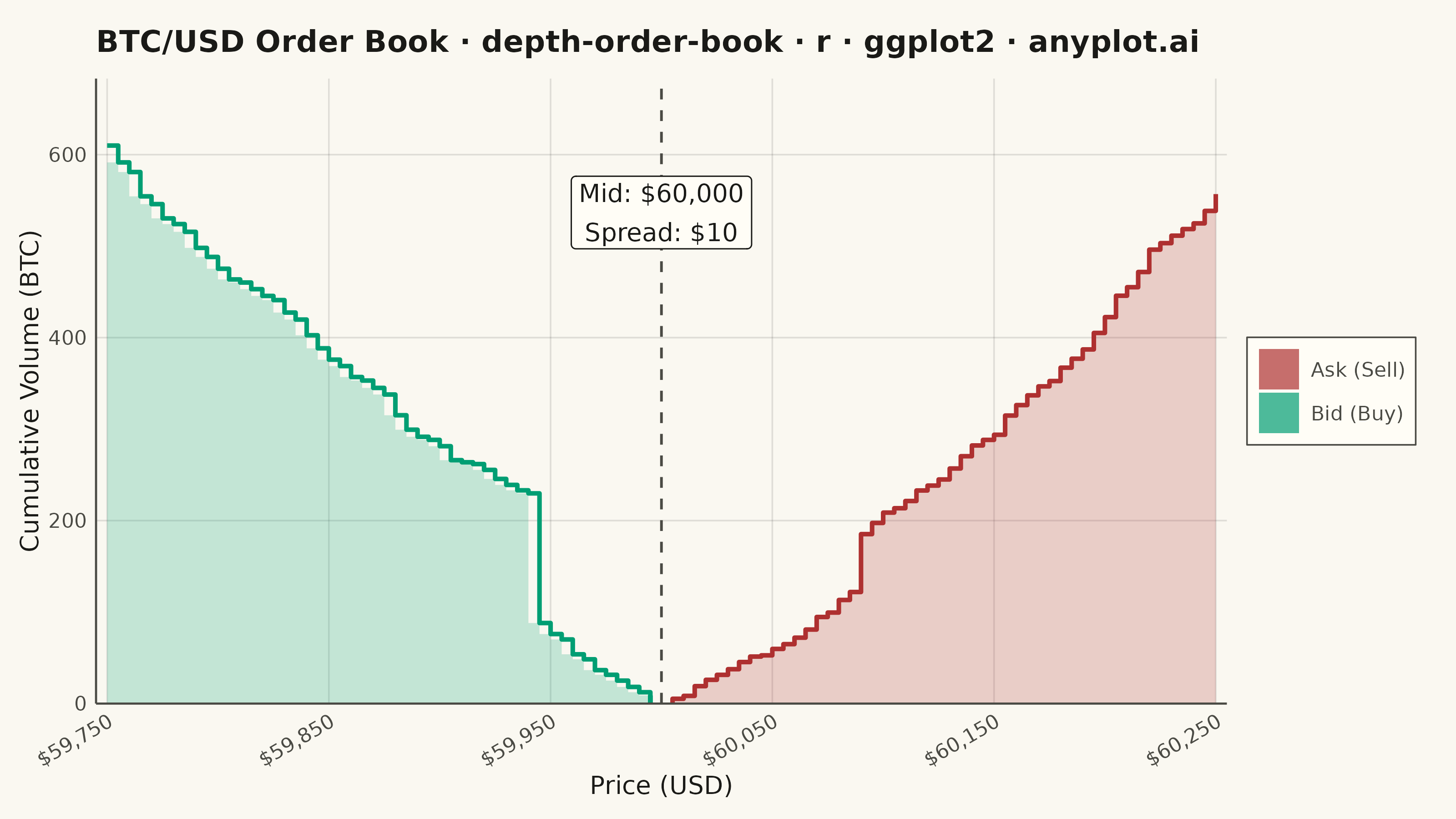
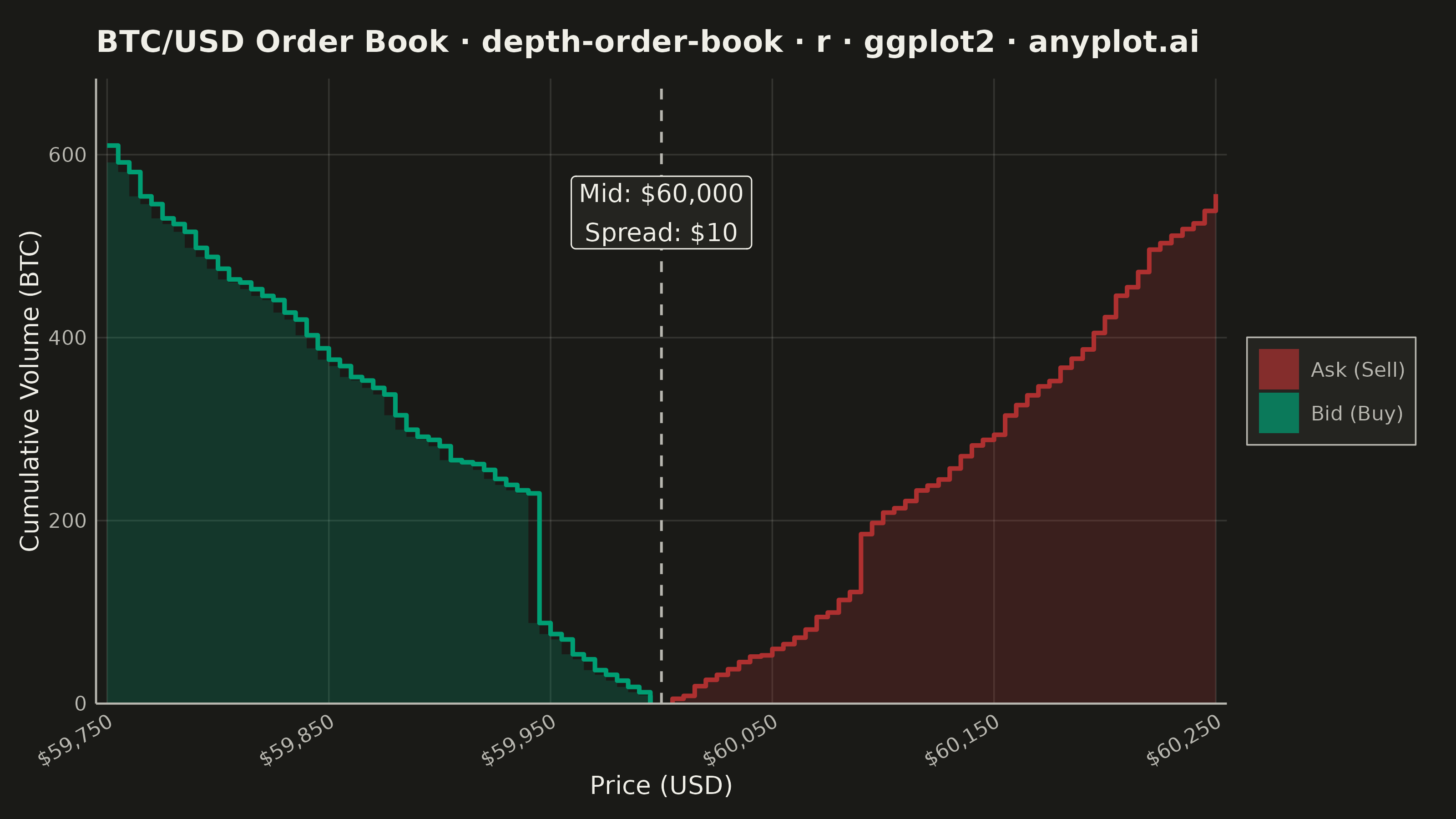
A market depth chart visualizes a snapshot of an exchange order book as two cumulative step areas around the mid price. Cumulative bid volume rises as a green step area to the left of the mid price (summing buy orders from the best bid downward), while cumulative ask volume rises as a red step area to the right (summing sell orders from the best ask upward). The bid-ask spread appears as a gap at the center, with price on the x-axis and cumulative quantity on the y-axis. This is the iconic chart found in nearly every trading and crypto exchange UI, revealing liquidity, support/resistance walls, and the imbalance between buying and selling pressure.
#' anyplot.ai
#' depth-order-book: Order Book Depth Chart
#' Library: ggplot2 3.5.1 | R 4.4.1
#' Quality: 86/100 | Created: 2026-06-15

library(ggplot2)
library(scales)
library(ragg)

set.seed(42)

# Theme tokens
THEME       <- Sys.getenv("ANYPLOT_THEME", "light")
PAGE_BG     <- if (THEME == "light") "#FAF8F1" else "#1A1A17"
ELEVATED_BG <- if (THEME == "light") "#FFFDF6" else "#242420"
INK         <- if (THEME == "light") "#1A1A17" else "#F0EFE8"
INK_SOFT    <- if (THEME == "light") "#4A4A44" else "#B8B7B0"

# Imprint palette — semantic: green = bids (buy), red = asks (sell)
BID_COLOR <- "#009E73"  # Imprint position 1 (brand green)
ASK_COLOR <- "#AE3030"  # Imprint position 5 (semantic: sell/loss)
GRID_COL  <- adjustcolor(INK, alpha.f = 0.12)

# Market parameters: BTC/USD snapshot near $60,000
mid_price   <- 60000
half_spread <- 5        # $10 total spread
n_levels    <- 50
tick_size   <- 5        # $5 between price levels

# Price grids — index 1 = best (closest to mid), index 50 = worst
bid_prices <- mid_price - half_spread - (seq_len(n_levels) - 1) * tick_size
ask_prices <- mid_price + half_spread + (seq_len(n_levels) - 1) * tick_size

# Individual order sizes with mild trend (deeper levels accumulate more liquidity)
qty_trend <- 1 + (seq_len(n_levels) - 1) * 0.04
bid_qtys  <- rlnorm(n_levels, meanlog = 1.5, sdlog = 0.5) * qty_trend
ask_qtys  <- rlnorm(n_levels, meanlog = 1.5, sdlog = 0.5) * qty_trend

# Insert liquidity walls — large resting orders that act as support/resistance
bid_qtys[12] <- bid_qtys[12] * 7
ask_qtys[18] <- ask_qtys[18] * 5

# Cumulative volume from mid price outward
bid_cum <- cumsum(bid_qtys)
ask_cum <- cumsum(ask_qtys)

# Build step polygon data — vectorized, no loops
make_step_poly <- function(prices, cums, side_label) {
    n  <- length(prices)
    xs <- rep(prices, each = 2)
    ys <- c(0, rep(cums, each = 2))[seq_len(2 * n)]
    data.frame(
        x    = c(xs, prices[n], prices[1]),
        y    = c(ys, 0, 0),
        side = side_label
    )
}

bid_poly <- make_step_poly(bid_prices, bid_cum, "Bid (Buy)")
ask_poly <- make_step_poly(ask_prices, ask_cum, "Ask (Sell)")
order_book <- rbind(bid_poly, ask_poly)

# Step outline data for geom_step — prepend (best_price, 0) for clean initial vertical
bid_step <- data.frame(
    price   = c(bid_prices[1], bid_prices),
    cum_vol = c(0, bid_cum),
    side    = "Bid (Buy)"
)
ask_step <- data.frame(
    price   = c(ask_prices[1], ask_prices),
    cum_vol = c(0, ask_cum),
    side    = "Ask (Sell)"
)
depth_df <- rbind(bid_step, ask_step)

max_cum    <- max(bid_cum[n_levels], ask_cum[n_levels])
label_text <- sprintf("Mid: $%s\nSpread: $%d",
                      format(mid_price, big.mark = ",", scientific = FALSE),
                      half_spread * 2)

plot_title <- "BTC/USD Order Book · depth-order-book · r · ggplot2 · anyplot.ai"
title_size <- max(8, round(12 * 67 / max(nchar(plot_title), 67)))

p <- ggplot() +
    geom_polygon(
        data  = order_book,
        aes(x = x, y = y, fill = side, group = side),
        color = NA, alpha = 0.22
    ) +
    geom_step(
        data      = depth_df,
        aes(x = price, y = cum_vol, color = side, group = side),
        direction = "hv", linewidth = 0.85
    ) +
    geom_vline(
        xintercept = mid_price,
        linetype = "dashed", color = INK_SOFT, linewidth = 0.5
    ) +
    annotate(
        "label",
        x = mid_price, y = max_cum * 0.88,
        label = label_text, color = INK, size = 3.5,
        hjust = 0.5, lineheight = 1.3,
        fill = ELEVATED_BG, label.size = 0.25
    ) +
    scale_fill_manual(
        name   = NULL,
        values = c("Bid (Buy)" = BID_COLOR, "Ask (Sell)" = ASK_COLOR),
        guide  = guide_legend(override.aes = list(alpha = 0.7))
    ) +
    scale_color_manual(
        name   = NULL,
        values = c("Bid (Buy)" = BID_COLOR, "Ask (Sell)" = ASK_COLOR),
        guide  = "none"
    ) +
    scale_x_continuous(
        labels = label_dollar(accuracy = 1),
        breaks = seq(59750, 60250, by = 100),
        expand = expansion(mult = 0.01)
    ) +
    scale_y_continuous(
        labels = label_comma(accuracy = 1),
        limits = c(0, max_cum * 1.12),
        expand = expansion(mult = c(0, 0))
    ) +
    labs(
        title = plot_title,
        x     = "Price (USD)",
        y     = "Cumulative Volume (BTC)"
    ) +
    theme_minimal(base_size = 8) +
    theme(
        plot.background   = element_rect(fill = PAGE_BG,  color = PAGE_BG),
        panel.background  = element_rect(fill = PAGE_BG,  color = NA),
        panel.grid.major  = element_line(color = GRID_COL, linewidth = 0.3),
        panel.grid.minor  = element_blank(),
        panel.border      = element_blank(),
        axis.line         = element_line(color = INK_SOFT, linewidth = 0.4),
        axis.title        = element_text(color = INK,      size = 10),
        axis.text         = element_text(color = INK_SOFT, size = 8),
        axis.text.x       = element_text(color = INK_SOFT, size = 8,
                                         angle = 30, hjust = 1),
        plot.title        = element_text(color = INK, size = title_size,
                                         face = "bold", margin = margin(b = 8)),
        legend.background = element_rect(fill = ELEVATED_BG, color = INK_SOFT,
                                         linewidth = 0.3),
        legend.text       = element_text(color = INK_SOFT, size = 8),
        legend.key        = element_rect(fill = NA, color = NA),
        plot.margin       = margin(t = 12, r = 16, b = 8, l = 8)
    )

ggsave(
    filename = sprintf("plot-%s.png", THEME),
    plot     = p,
    device   = ragg::agg_png,
    width    = 8,
    height   = 4.5,
    units    = "in",
    dpi      = 400
)
Runnable source as JSON, for any HTTP client: https://api.anyplot.ai/specs/depth-order-book/ggplot2/code. Any spec id and library id listed in llms-full.txt fit the same URL shape; every URL below is complete and callable.
{
  "spec_id": "depth-order-book",
  "language": "r",
  "library": "ggplot2",
  "page": "https://anyplot.ai/depth-order-book/r/ggplot2",
  "hub": "https://anyplot.ai/depth-order-book",
  "code_json": "https://api.anyplot.ai/specs/depth-order-book/ggplot2/code",
  "spec_json": "https://api.anyplot.ai/specs/depth-order-book",
  "render_light_png": "https://storage.googleapis.com/anyplot-images/plots/depth-order-book/r/ggplot2/plot-light.png",
  "render_dark_png": "https://storage.googleapis.com/anyplot-images/plots/depth-order-book/r/ggplot2/plot-dark.png",
  "quality_score": 86.0,
  "license": "MIT",
  "guide": "https://anyplot.ai/llms.txt"
}
Part of Order Book Depth Chart on anyplot.ai.