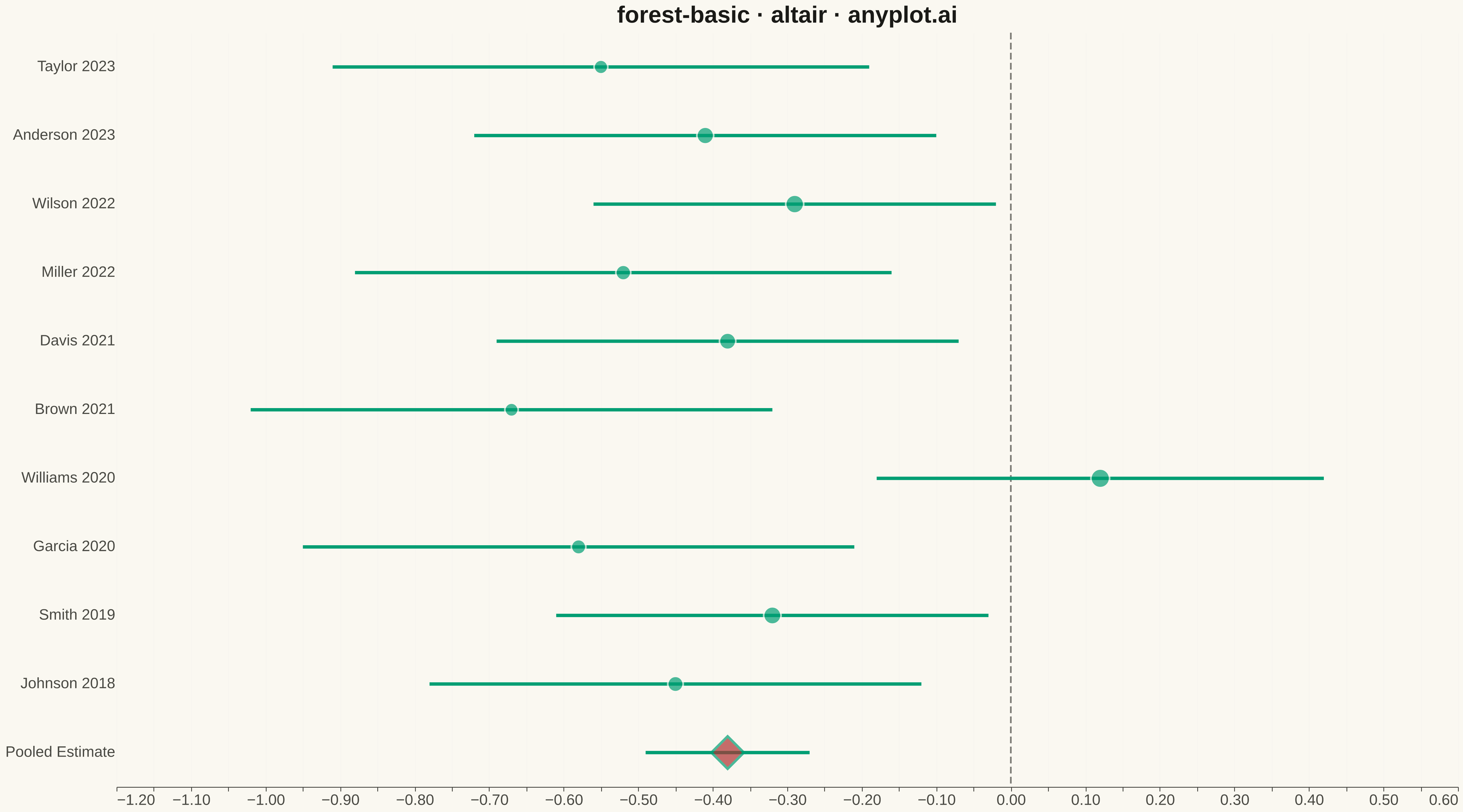
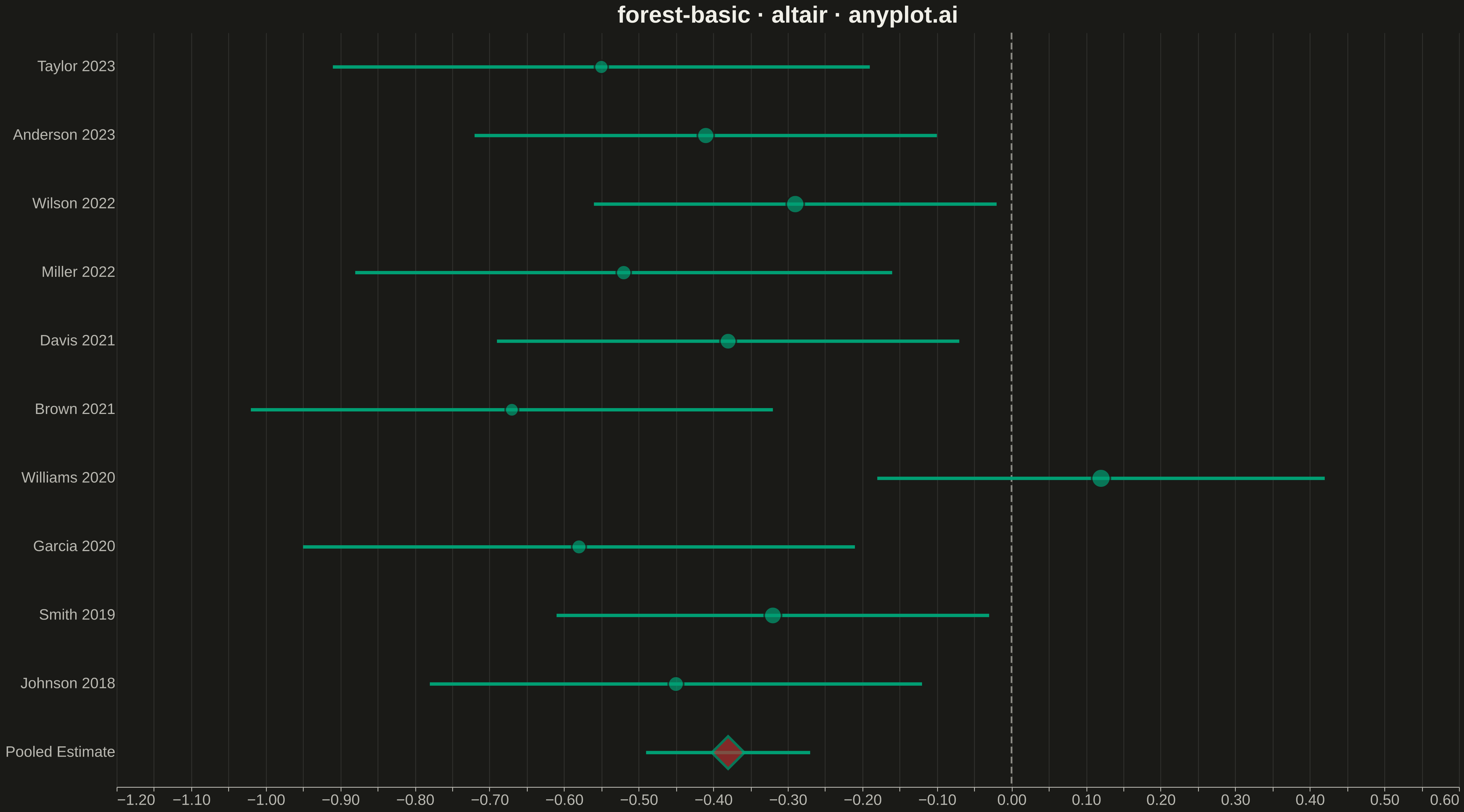
A forest plot displays effect sizes with confidence intervals from multiple studies in a meta-analysis. Each study is represented as a point estimate with horizontal whiskers showing the confidence interval, and a diamond at the bottom shows the pooled estimate. The plot includes a vertical reference line at the null effect (typically 0 or 1), making it easy to assess statistical significance and heterogeneity across studies.
""" anyplot.ai
forest-basic: Meta-Analysis Forest Plot
Library: altair 6.1.0 | Python 3.13.13
Quality: 94/100 | Updated: 2026-05-11
"""

import os

import altair as alt
import pandas as pd


# Theme tokens
THEME = os.getenv("ANYPLOT_THEME", "light")
PAGE_BG = "#FAF8F1" if THEME == "light" else "#1A1A17"
ELEVATED_BG = "#FFFDF6" if THEME == "light" else "#242420"
INK = "#1A1A17" if THEME == "light" else "#F0EFE8"
INK_SOFT = "#4A4A44" if THEME == "light" else "#B8B7B0"
INK_MUTED = "#6B6A63" if THEME == "light" else "#A8A79F"

# Data: Meta-analysis of RCTs comparing treatment efficacy
studies = [
    "Johnson 2018",
    "Smith 2019",
    "Garcia 2020",
    "Williams 2020",
    "Brown 2021",
    "Davis 2021",
    "Miller 2022",
    "Wilson 2022",
    "Anderson 2023",
    "Taylor 2023",
]

effect_sizes = [-0.45, -0.32, -0.58, 0.12, -0.67, -0.38, -0.52, -0.29, -0.41, -0.55]
ci_lower = [-0.78, -0.61, -0.95, -0.18, -1.02, -0.69, -0.88, -0.56, -0.72, -0.91]
ci_upper = [-0.12, -0.03, -0.21, 0.42, -0.32, -0.07, -0.16, -0.02, -0.10, -0.19]
weights = [8.5, 10.2, 7.8, 11.5, 6.9, 9.3, 8.1, 10.8, 9.7, 7.2]

# Pooled estimate
pooled_effect = -0.38
pooled_ci_lower = -0.49
pooled_ci_upper = -0.27

# Order labels for y-axis (studies at top, pooled estimate at bottom)
y_labels = list(reversed(studies)) + ["Pooled Estimate"]

# Create DataFrame for studies
df_studies = pd.DataFrame(
    {"study": studies, "effect_size": effect_sizes, "ci_lower": ci_lower, "ci_upper": ci_upper, "weight": weights}
)

# Normalize weights for marker sizing
weight_min = min(weights)
weight_max = max(weights)
df_studies["marker_size"] = 150 + (df_studies["weight"] - weight_min) / (weight_max - weight_min) * 350

# Create DataFrame for pooled estimate
df_pooled = pd.DataFrame(
    {
        "study": ["Pooled Estimate"],
        "effect_size": [pooled_effect],
        "ci_lower": [pooled_ci_lower],
        "ci_upper": [pooled_ci_upper],
    }
)

# Vertical reference line at null effect (0)
reference_line = (
    alt.Chart(pd.DataFrame({"x": [0]}))
    .mark_rule(color=INK_SOFT, strokeDash=[8, 4], strokeWidth=2, opacity=0.7)
    .encode(x="x:Q")
)

# Confidence interval lines for studies
ci_lines = (
    alt.Chart(df_studies)
    .mark_rule(color="#009E73", strokeWidth=4)
    .encode(
        x=alt.X("ci_lower:Q", scale=alt.Scale(domain=[-1.15, 0.60])), x2="ci_upper:Q", y=alt.Y("study:N", sort=y_labels)
    )
)

# Effect size points for studies
points = (
    alt.Chart(df_studies)
    .mark_point(filled=True, color="#009E73", stroke=PAGE_BG, strokeWidth=2)
    .encode(
        x=alt.X("effect_size:Q", scale=alt.Scale(domain=[-1.15, 0.60])),
        y=alt.Y("study:N", sort=y_labels),
        size=alt.Size("marker_size:Q", legend=None, scale=alt.Scale(range=[150, 500])),
        tooltip=[
            alt.Tooltip("study:N", title="Study"),
            alt.Tooltip("effect_size:Q", title="Effect Size", format=".2f"),
            alt.Tooltip("ci_lower:Q", title="CI Lower", format=".2f"),
            alt.Tooltip("ci_upper:Q", title="CI Upper", format=".2f"),
        ],
    )
)

# Pooled estimate confidence interval line
pooled_ci = (
    alt.Chart(df_pooled)
    .mark_rule(color="#009E73", strokeWidth=4)
    .encode(
        x=alt.X("ci_lower:Q", scale=alt.Scale(domain=[-1.15, 0.60])), x2="ci_upper:Q", y=alt.Y("study:N", sort=y_labels)
    )
)

# Diamond marker for pooled estimate
pooled_diamond = (
    alt.Chart(df_pooled)
    .mark_point(shape="diamond", filled=True, size=1500, color="#AE3030", stroke="#009E73", strokeWidth=3)
    .encode(
        x=alt.X("effect_size:Q", scale=alt.Scale(domain=[-1.15, 0.60])),
        y=alt.Y("study:N", sort=y_labels),
        tooltip=[
            alt.Tooltip("study:N", title="Estimate"),
            alt.Tooltip("effect_size:Q", title="Effect Size", format=".2f"),
            alt.Tooltip("ci_lower:Q", title="CI Lower", format=".2f"),
            alt.Tooltip("ci_upper:Q", title="CI Upper", format=".2f"),
        ],
    )
)

# Combine all layers
chart = (
    alt.layer(reference_line, ci_lines, points, pooled_ci, pooled_diamond)
    .properties(
        width=1600,
        height=900,
        background=PAGE_BG,
        title=alt.Title("forest-basic · altair · anyplot.ai", fontSize=28, anchor="middle"),
    )
    .configure_axis(
        labelFontSize=18,
        titleFontSize=22,
        domainColor=INK_SOFT,
        tickColor=INK_SOFT,
        labelColor=INK_SOFT,
        titleColor=INK,
    )
    .configure_axisX(title="Standardized Mean Difference (95% CI)", grid=True, gridOpacity=0.10)
    .configure_axisY(title=None, grid=False, ticks=False, domain=False)
    .configure_title(color=INK)
    .configure_view(strokeWidth=0, fill=PAGE_BG)
)

# Save as PNG and HTML with theme-suffixed names
chart.save(f"plot-{THEME}.png", scale_factor=3.0)
chart.save(f"plot-{THEME}.html")
Runnable source as JSON, for any HTTP client: https://api.anyplot.ai/specs/forest-basic/altair/code. Any spec id and library id listed in llms-full.txt fit the same URL shape; every URL below is complete and callable.
{
  "spec_id": "forest-basic",
  "language": "python",
  "library": "altair",
  "page": "https://anyplot.ai/forest-basic/python/altair",
  "hub": "https://anyplot.ai/forest-basic",
  "code_json": "https://api.anyplot.ai/specs/forest-basic/altair/code",
  "spec_json": "https://api.anyplot.ai/specs/forest-basic",
  "render_light_png": "https://storage.googleapis.com/anyplot-images/plots/forest-basic/python/altair/plot-light.png",
  "render_dark_png": "https://storage.googleapis.com/anyplot-images/plots/forest-basic/python/altair/plot-dark.png",
  "interactive_light_html": "https://storage.googleapis.com/anyplot-images/plots/forest-basic/python/altair/plot-light.html",
  "interactive_dark_html": "https://storage.googleapis.com/anyplot-images/plots/forest-basic/python/altair/plot-dark.html",
  "quality_score": 94.0,
  "license": "MIT",
  "guide": "https://anyplot.ai/llms.txt"
}
Part of Meta-Analysis Forest Plot on anyplot.ai.