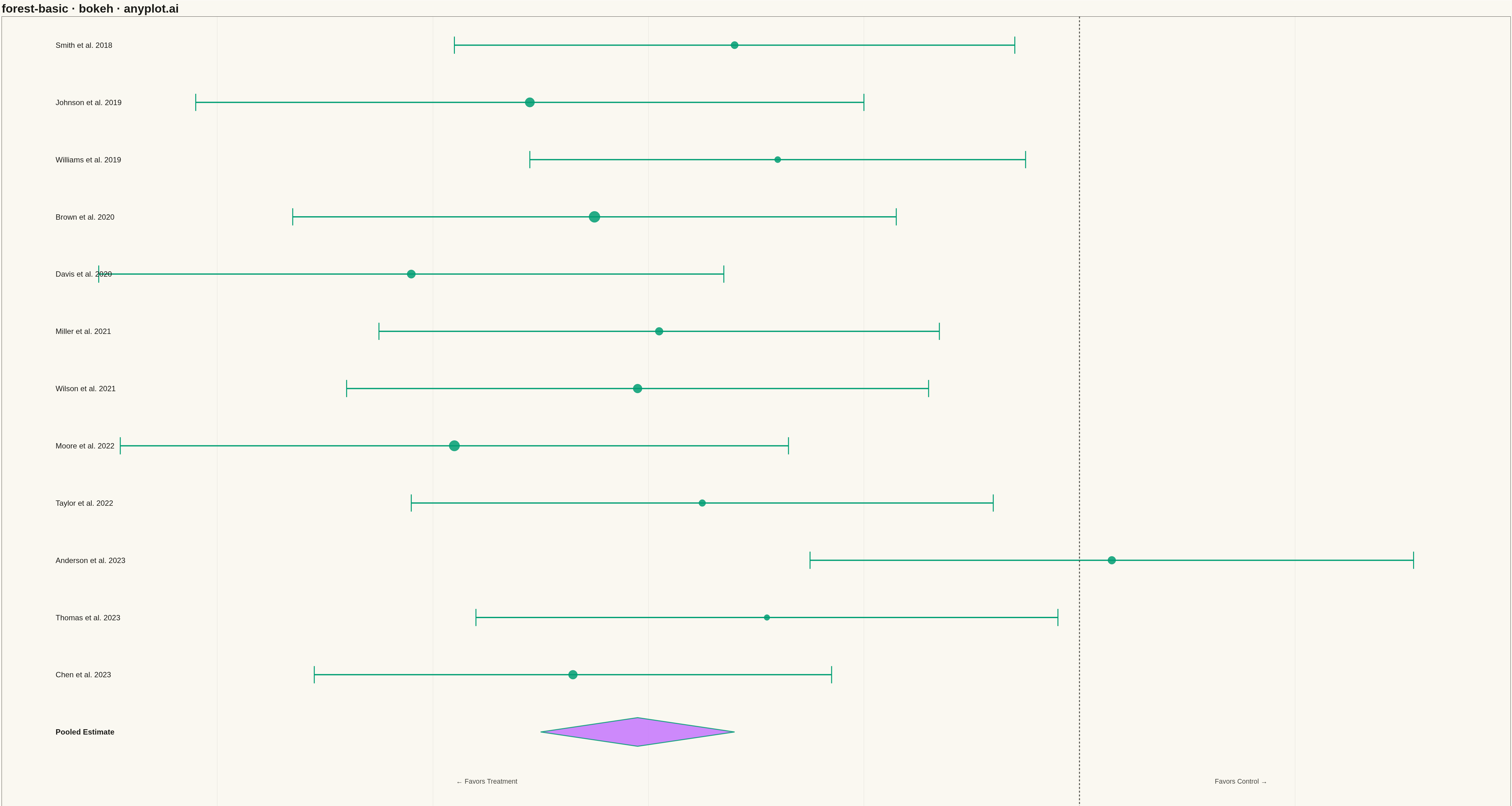
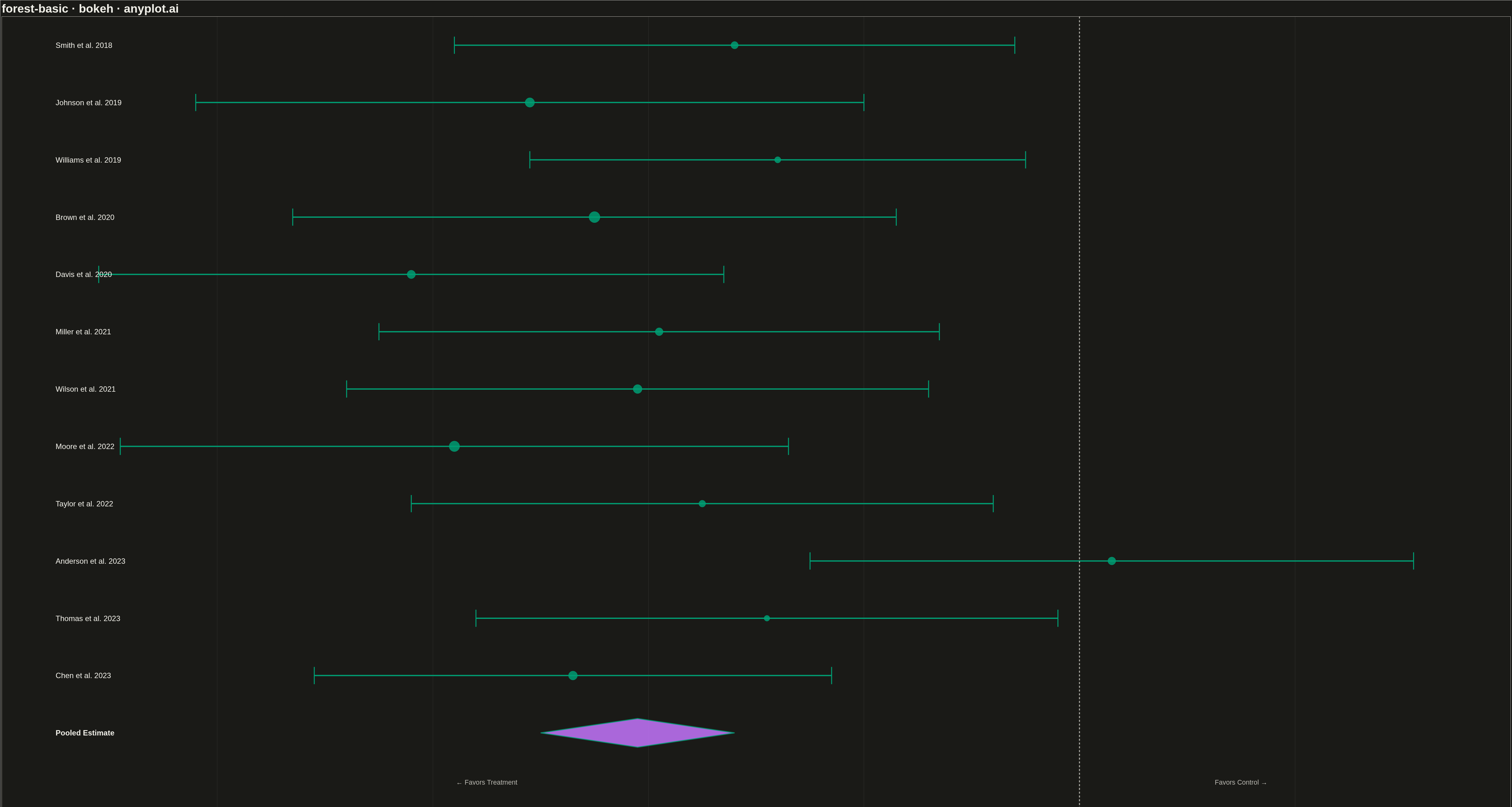
A forest plot displays effect sizes with confidence intervals from multiple studies in a meta-analysis. Each study is represented as a point estimate with horizontal whiskers showing the confidence interval, and a diamond at the bottom shows the pooled estimate. The plot includes a vertical reference line at the null effect (typically 0 or 1), making it easy to assess statistical significance and heterogeneity across studies.
""" anyplot.ai
forest-basic: Meta-Analysis Forest Plot
Library: bokeh 3.9.0 | Python 3.13.13
Quality: 90/100 | Updated: 2026-05-11
"""

import os
import sys
from pathlib import Path


# Remove local directory from sys.path to avoid importing local bokeh.py
sys.path = [p for p in sys.path if not p.startswith(str(Path(__file__).parent))]

import time

import numpy as np
from bokeh.io import output_file, save
from bokeh.models import ColumnDataSource, HoverTool, Label, Span
from bokeh.plotting import figure
from selenium import webdriver
from selenium.webdriver.chrome.options import Options


THEME = os.getenv("ANYPLOT_THEME", "light")

# Theme-adaptive colors
PAGE_BG = "#FAF8F1" if THEME == "light" else "#1A1A17"
INK = "#1A1A17" if THEME == "light" else "#F0EFE8"
INK_SOFT = "#4A4A44" if THEME == "light" else "#B8B7B0"

# Okabe-Ito palette
BRAND = "#009E73"
SECONDARY = "#C475FD"

# Data - Meta-analysis of blood pressure reduction trials
np.random.seed(42)

studies = [
    "Smith et al. 2018",
    "Johnson et al. 2019",
    "Williams et al. 2019",
    "Brown et al. 2020",
    "Davis et al. 2020",
    "Miller et al. 2021",
    "Wilson et al. 2021",
    "Moore et al. 2022",
    "Taylor et al. 2022",
    "Anderson et al. 2023",
    "Thomas et al. 2023",
    "Chen et al. 2023",
    "Pooled Estimate",
]

# Effect sizes (mean difference in mmHg) with confidence intervals
# Added study crossing null line for better forest plot demonstration
effect_sizes = np.array([-3.2, -5.1, -2.8, -4.5, -6.2, -3.9, -4.1, -5.8, -3.5, 0.3, -2.9, -4.7, -4.1])
ci_lower = np.array([-5.8, -8.2, -5.1, -7.3, -9.1, -6.5, -6.8, -8.9, -6.2, -2.5, -5.6, -7.1, -5.0])
ci_upper = np.array([-0.6, -2.0, -0.5, -1.7, -3.3, -1.3, -1.4, -2.7, -0.8, 3.1, -0.2, -2.3, -3.2])

# Weights based on sample size
weights = np.array([8, 12, 6, 15, 10, 9, 11, 14, 7, 9, 5, 11, 22])

# Y positions (reversed so first study is at top)
y_positions = list(range(len(studies) - 1, -1, -1))

# Create figure
p = figure(
    width=4800,
    height=2700,
    title="forest-basic · bokeh · anyplot.ai",
    x_axis_label="Mean Difference in Blood Pressure (mmHg)",
    y_range=(-1.5, len(studies) - 0.5),
    x_range=(-10, 4),
    tools="pan,wheel_zoom,reset",
    toolbar_location="below",
)

# Add vertical reference line at null effect (0)
null_line = Span(location=0, dimension="height", line_color=INK_SOFT, line_width=3, line_dash="dashed")
p.add_layout(null_line)

# Prepare data for individual studies (excluding pooled estimate)
study_source = ColumnDataSource(
    data={
        "study": studies[:-1],
        "effect": effect_sizes[:-1],
        "ci_lower": ci_lower[:-1],
        "ci_upper": ci_upper[:-1],
        "y": y_positions[:-1],
        "size": (weights[:-1] / weights[:-1].max() * 25 + 10).tolist(),
    }
)

# Draw confidence interval lines (whiskers)
for i in range(len(studies) - 1):
    p.line(x=[ci_lower[i], ci_upper[i]], y=[y_positions[i], y_positions[i]], line_width=4, line_color=BRAND)
    # Add CI end caps
    p.line(
        x=[ci_lower[i], ci_lower[i]], y=[y_positions[i] - 0.15, y_positions[i] + 0.15], line_width=3, line_color=BRAND
    )
    p.line(
        x=[ci_upper[i], ci_upper[i]], y=[y_positions[i] - 0.15, y_positions[i] + 0.15], line_width=3, line_color=BRAND
    )

# Plot effect size points (size proportional to weight)
p.scatter(x="effect", y="y", source=study_source, size="size", color=BRAND, alpha=0.85)

# Add HoverTool for interactivity
hover = HoverTool(
    tooltips=[("Study", "@study"), ("Effect Size", "@effect{0.0}"), ("95% CI", "[@ci_lower{0.0}, @ci_upper{0.0}]")]
)
p.add_tools(hover)

# Add study labels on the left
for i, study in enumerate(studies[:-1]):
    label = Label(
        x=-9.5,
        y=y_positions[i],
        text=study,
        text_font_size="18pt",
        text_align="left",
        text_baseline="middle",
        text_color=INK,
    )
    p.add_layout(label)

# Draw pooled estimate as a diamond
pooled_y = y_positions[-1]
pooled_effect = effect_sizes[-1]
pooled_lower = ci_lower[-1]
pooled_upper = ci_upper[-1]

# Diamond vertices
diamond_x = [pooled_lower, pooled_effect, pooled_upper, pooled_effect, pooled_lower]
diamond_y = [pooled_y, pooled_y + 0.25, pooled_y, pooled_y - 0.25, pooled_y]

p.patch(x=diamond_x, y=diamond_y, fill_color=SECONDARY, line_color=BRAND, line_width=3, alpha=0.85)

# Add pooled estimate label
pooled_label = Label(
    x=-9.5,
    y=pooled_y,
    text="Pooled Estimate",
    text_font_size="18pt",
    text_font_style="bold",
    text_align="left",
    text_baseline="middle",
    text_color=INK,
)
p.add_layout(pooled_label)

# Add "Favors Treatment" and "Favors Control" labels
favors_treatment = Label(
    x=-5.5,
    y=-0.8,
    text="← Favors Treatment",
    text_font_size="16pt",
    text_align="center",
    text_baseline="top",
    text_color=INK_SOFT,
)
p.add_layout(favors_treatment)

favors_control = Label(
    x=1.5,
    y=-0.8,
    text="Favors Control →",
    text_font_size="16pt",
    text_align="center",
    text_baseline="top",
    text_color=INK_SOFT,
)
p.add_layout(favors_control)

# Styling
p.title.text_font_size = "28pt"
p.title.text_color = INK
p.xaxis.axis_label_text_font_size = "22pt"
p.yaxis.axis_label_text_font_size = "22pt"
p.xaxis.major_label_text_font_size = "18pt"
p.yaxis.major_label_text_font_size = "18pt"

# Color styling
p.xaxis.axis_label_text_color = INK
p.yaxis.axis_label_text_color = INK
p.xaxis.major_label_text_color = INK_SOFT
p.yaxis.major_label_text_color = INK_SOFT
p.xaxis.axis_line_color = INK_SOFT
p.yaxis.axis_line_color = INK_SOFT
p.xaxis.major_tick_line_color = INK_SOFT
p.yaxis.major_tick_line_color = INK_SOFT

# Hide y-axis ticks and labels (studies are labeled manually)
p.yaxis.visible = False

# Grid styling
p.xgrid.grid_line_color = INK
p.xgrid.grid_line_alpha = 0.10
p.ygrid.grid_line_color = None

# Background
p.background_fill_color = PAGE_BG
p.border_fill_color = PAGE_BG
p.outline_line_color = INK_SOFT

# Save HTML
output_file(f"plot-{THEME}.html")
save(p)

# Screenshot with headless Chrome via Selenium
W, H = 4800, 2700
opts = Options()
for arg in (
    "--headless=new",
    "--no-sandbox",
    "--disable-dev-shm-usage",
    "--disable-gpu",
    f"--window-size={W},{H}",
    "--hide-scrollbars",
):
    opts.add_argument(arg)

driver = webdriver.Chrome(options=opts)
driver.set_window_size(W, H)
driver.get(f"file://{Path(f'plot-{THEME}.html').resolve()}")
time.sleep(3)
driver.save_screenshot(f"plot-{THEME}.png")
driver.quit()
Runnable source as JSON, for any HTTP client: https://api.anyplot.ai/specs/forest-basic/bokeh/code. Any spec id and library id listed in llms-full.txt fit the same URL shape; every URL below is complete and callable.
{
  "spec_id": "forest-basic",
  "language": "python",
  "library": "bokeh",
  "page": "https://anyplot.ai/forest-basic/python/bokeh",
  "hub": "https://anyplot.ai/forest-basic",
  "code_json": "https://api.anyplot.ai/specs/forest-basic/bokeh/code",
  "spec_json": "https://api.anyplot.ai/specs/forest-basic",
  "render_light_png": "https://storage.googleapis.com/anyplot-images/plots/forest-basic/python/bokeh/plot-light.png",
  "render_dark_png": "https://storage.googleapis.com/anyplot-images/plots/forest-basic/python/bokeh/plot-dark.png",
  "interactive_light_html": "https://storage.googleapis.com/anyplot-images/plots/forest-basic/python/bokeh/plot-light.html",
  "interactive_dark_html": "https://storage.googleapis.com/anyplot-images/plots/forest-basic/python/bokeh/plot-dark.html",
  "quality_score": 90.0,
  "license": "MIT",
  "guide": "https://anyplot.ai/llms.txt"
}
Part of Meta-Analysis Forest Plot on anyplot.ai.