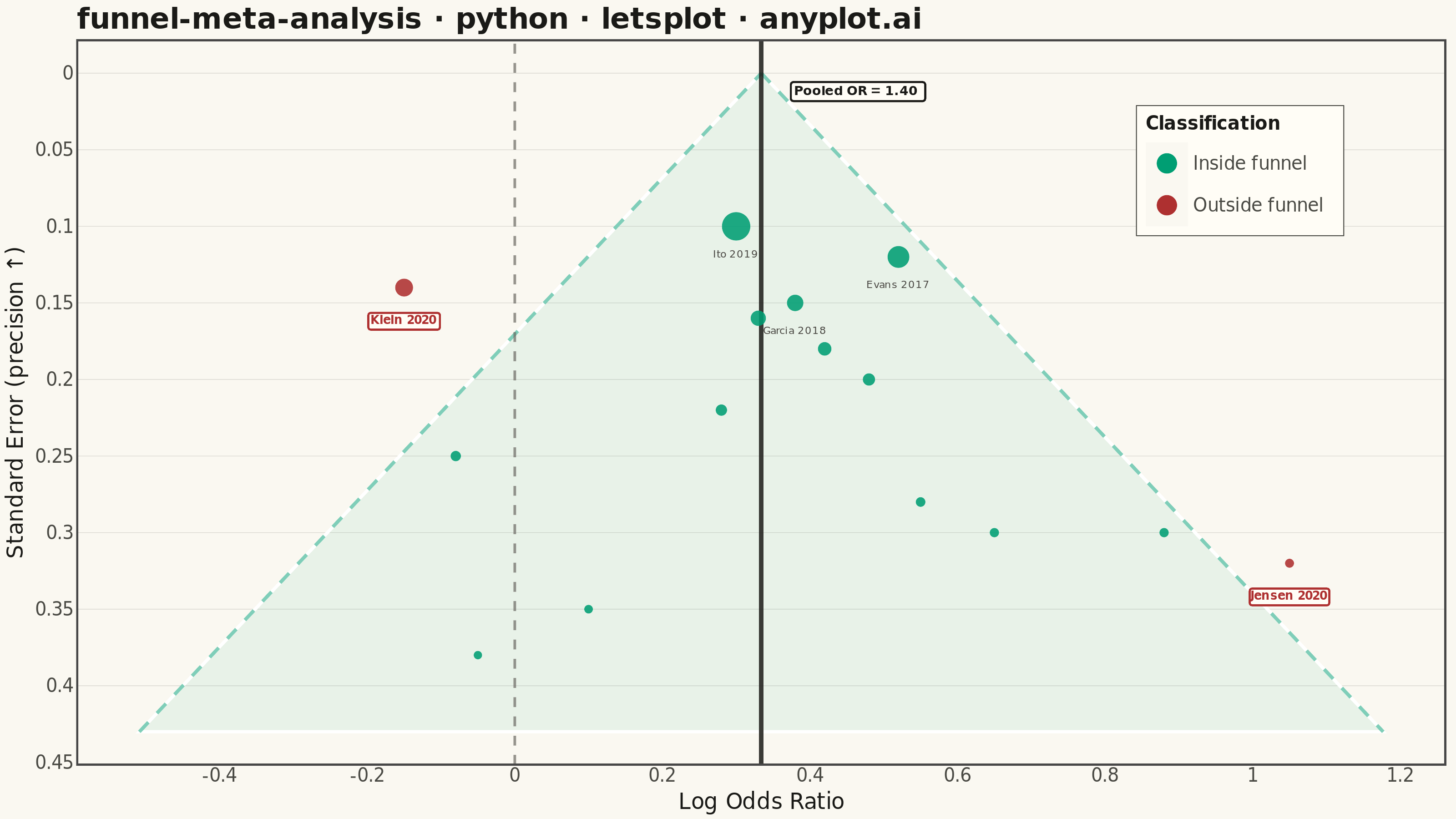
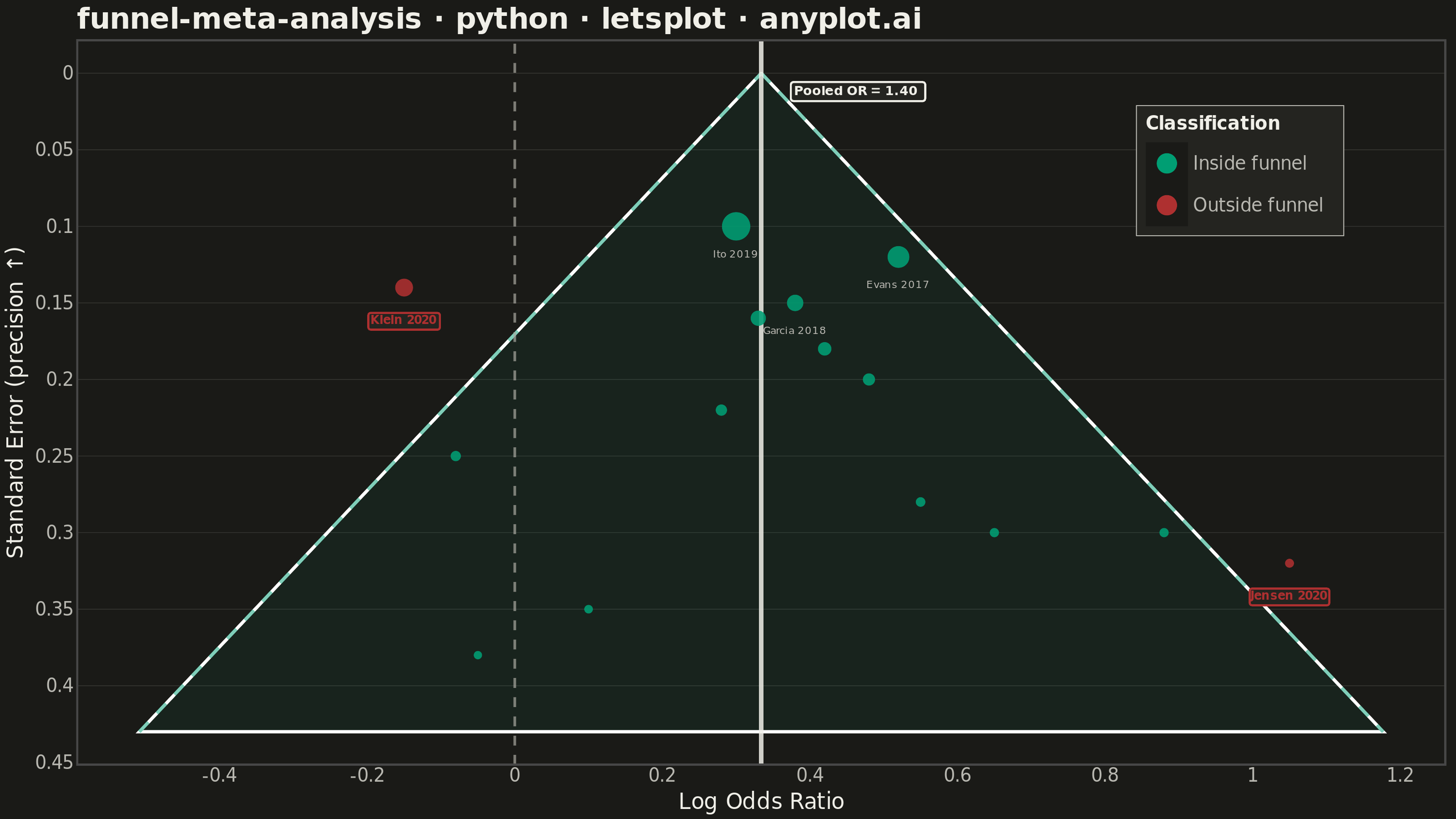
A funnel plot used in meta-analysis to assess publication bias by plotting individual study effect sizes against their precision (typically standard error). Studies scatter around a summary effect line, with pseudo 95% confidence limits forming an inverted funnel shape. In the absence of bias, studies distribute symmetrically around the summary effect; asymmetry suggests publication bias or systematic heterogeneity. This is a standard tool in systematic reviews and Cochrane-style meta-analyses.
""" anyplot.ai
funnel-meta-analysis: Meta-Analysis Funnel Plot for Publication Bias
Library: letsplot 4.10.1 | Python 3.13.13
Quality: 90/100 | Updated: 2026-06-10
"""

import os

import numpy as np
import pandas as pd
from lets_plot import *


LetsPlot.setup_html()

THEME = os.getenv("ANYPLOT_THEME", "light")
PAGE_BG = "#FAF8F1" if THEME == "light" else "#1A1A17"
ELEVATED_BG = "#FFFDF6" if THEME == "light" else "#242420"
INK = "#1A1A17" if THEME == "light" else "#F0EFE8"
INK_SOFT = "#4A4A44" if THEME == "light" else "#B8B7B0"
INK_MUTED = "#6B6A63" if THEME == "light" else "#A8A79F"
GRID_COLOR = "#D9D7D0" if THEME == "light" else "#3A3A36"

# Imprint palette — first series always #009E73
BRAND = "#009E73"  # Inside funnel (expected, within confidence limits)
OUTLIER = "#AE3030"  # Outside funnel — semantic anchor: potential bias / outlier

# Data: Meta-analysis of 15 RCTs comparing drug vs placebo
# Effect sizes are log odds ratios; null effect at 0
studies = [
    {"study": "Adams 2015", "effect_size": 0.42, "std_error": 0.18, "n": 120},
    {"study": "Baker 2016", "effect_size": 0.28, "std_error": 0.22, "n": 85},
    {"study": "Chen 2016", "effect_size": 0.65, "std_error": 0.30, "n": 48},
    {"study": "Davis 2017", "effect_size": -0.08, "std_error": 0.25, "n": 64},
    {"study": "Evans 2017", "effect_size": 0.52, "std_error": 0.12, "n": 280},
    {"study": "Foster 2018", "effect_size": 0.10, "std_error": 0.35, "n": 34},
    {"study": "Garcia 2018", "effect_size": 0.38, "std_error": 0.15, "n": 180},
    {"study": "Hughes 2019", "effect_size": 0.55, "std_error": 0.28, "n": 52},
    {"study": "Ito 2019", "effect_size": 0.30, "std_error": 0.10, "n": 410},
    {"study": "Jensen 2020", "effect_size": 1.05, "std_error": 0.32, "n": 40},
    {"study": "Klein 2020", "effect_size": -0.15, "std_error": 0.14, "n": 205},
    {"study": "Lee 2021", "effect_size": 0.48, "std_error": 0.20, "n": 100},
    {"study": "Morgan 2021", "effect_size": 0.33, "std_error": 0.16, "n": 160},
    {"study": "Nguyen 2022", "effect_size": 0.88, "std_error": 0.30, "n": 46},
    {"study": "Olsen 2023", "effect_size": -0.05, "std_error": 0.38, "n": 28},
]

df = pd.DataFrame(studies)

# Inverse-variance weights and pooled effect estimate
weights = 1 / df["std_error"] ** 2
pooled_effect = (df["effect_size"] * weights).sum() / weights.sum()
df["iw"] = weights

# Classify studies: inside or outside the 95% funnel boundary
df["position"] = np.where(
    (df["effect_size"] >= pooled_effect - 1.96 * df["std_error"])
    & (df["effect_size"] <= pooled_effect + 1.96 * df["std_error"]),
    "Inside funnel",
    "Outside funnel",
)

# Pseudo 95% confidence funnel boundary
se_max = df["std_error"].max() + 0.05
se_range = np.linspace(0, se_max, 200)
funnel_upper = pooled_effect + 1.96 * se_range
funnel_lower = pooled_effect - 1.96 * se_range

funnel_df = pd.DataFrame(
    {"x": np.concatenate([funnel_lower, funnel_upper[::-1]]), "y": np.concatenate([se_range, se_range[::-1]])}
)

funnel_lines_df = pd.DataFrame(
    {
        "x": np.concatenate([funnel_lower, funnel_upper]),
        "y": np.concatenate([se_range, se_range]),
        "side": ["lower"] * len(se_range) + ["upper"] * len(se_range),
    }
)

# Pooled OR annotation (single-row data frame for geom_label)
annotation_df = pd.DataFrame(
    {"x": [pooled_effect + 0.04], "y": [0.012], "label": [f"Pooled OR = {np.exp(pooled_effect):.2f}"]}
)

# Top 3 highest-weight inside-funnel studies for labeling
inside_top = df[df["position"] == "Inside funnel"].nlargest(3, "iw")

title = "funnel-meta-analysis · python · letsplot · anyplot.ai"
title_size = round(16 * min(1.0, 67 / len(title)))

plot = (
    ggplot()
    # Funnel confidence region (shaded polygon)
    + geom_polygon(aes(x="x", y="y"), data=funnel_df, fill=BRAND, alpha=0.07)
    # Funnel boundary lines (95% CI dashed)
    + geom_line(
        aes(x="x", y="y", group="side"), data=funnel_lines_df, color=BRAND, size=0.8, linetype="dashed", alpha=0.5
    )
    # Null effect reference line
    + geom_vline(xintercept=0, color=INK_MUTED, size=0.6, linetype="dashed", alpha=0.7)
    # Pooled effect line
    + geom_vline(xintercept=pooled_effect, color=INK, size=1.1, alpha=0.85)
    # Study points — sized by inverse-variance weight, colored by classification
    + geom_point(
        aes(x="effect_size", y="std_error", color="position", size="iw"),
        data=df,
        shape=16,
        alpha=0.88,
        tooltips=layer_tooltips()
        .title("@study")
        .line("Effect (log OR)|@effect_size{.3f}")
        .line("Std. error|@std_error{.3f}")
        .line("Sample size|@n")
        .line("Status|@position"),
    )
    + scale_color_manual(values={"Inside funnel": BRAND, "Outside funnel": OUTLIER}, name="Classification")
    + scale_size(range=[2.0, 7.0], guide="none")
    # Outlier labels with filled background — right-align Jensen 2020 to prevent canvas overflow
    + geom_label(
        aes(x="effect_size", y="std_error", label="study"),
        data=df[df["study"] == "Jensen 2020"],
        color=OUTLIER,
        fill=ELEVATED_BG,
        size=3.2,
        nudge_y=-0.022,
        hjust=1.1,
        fontface="bold",
        show_legend=False,
    )
    + geom_label(
        aes(x="effect_size", y="std_error", label="study"),
        data=df[df["study"] == "Klein 2020"],
        color=OUTLIER,
        fill=ELEVATED_BG,
        size=3.2,
        nudge_y=-0.022,
        hjust=-0.15,
        fontface="bold",
        show_legend=False,
    )
    # Top-weight inside-funnel study labels
    + geom_text(
        aes(x="effect_size", y="std_error", label="study"),
        data=inside_top,
        color=INK_SOFT,
        size=2.8,
        nudge_y=-0.018,
        show_legend=False,
    )
    # Pooled OR annotation box
    + geom_label(
        aes(x="x", y="y", label="label"),
        data=annotation_df,
        color=INK,
        fill=ELEVATED_BG,
        size=3.5,
        fontface="bold",
        hjust=0,
        show_legend=False,
    )
    # Inverted y-axis: lower SE (higher precision) at the top
    + scale_y_reverse()
    + labs(x="Log Odds Ratio", y="Standard Error (precision ↑)", title=title)
    + ggsize(800, 450)
    + theme_minimal()
    + theme(
        plot_title=element_text(size=title_size, face="bold", color=INK),
        axis_title=element_text(size=12, color=INK),
        axis_text=element_text(size=10, color=INK_SOFT),
        panel_grid_major_x=element_blank(),
        panel_grid_major_y=element_line(color=GRID_COLOR, size=0.3),
        panel_grid_minor=element_blank(),
        axis_line=element_line(color=INK_SOFT, size=0.4),
        legend_position=[0.85, 0.82],
        legend_title=element_text(size=10, face="bold", color=INK),
        legend_text=element_text(size=10, color=INK_SOFT),
        legend_background=element_rect(fill=ELEVATED_BG, color=INK_SOFT, size=0.5),
        plot_background=element_rect(fill=PAGE_BG, color=PAGE_BG),
        panel_background=element_rect(fill=PAGE_BG),
    )
)

ggsave(plot, f"plot-{THEME}.png", scale=4, path=".")
ggsave(plot, f"plot-{THEME}.html", path=".")
Runnable source as JSON, for any HTTP client: https://api.anyplot.ai/specs/funnel-meta-analysis/letsplot/code. Any spec id and library id listed in llms-full.txt fit the same URL shape; every URL below is complete and callable.
{
  "spec_id": "funnel-meta-analysis",
  "language": "python",
  "library": "letsplot",
  "page": "https://anyplot.ai/funnel-meta-analysis/python/letsplot",
  "hub": "https://anyplot.ai/funnel-meta-analysis",
  "code_json": "https://api.anyplot.ai/specs/funnel-meta-analysis/letsplot/code",
  "spec_json": "https://api.anyplot.ai/specs/funnel-meta-analysis",
  "render_light_png": "https://storage.googleapis.com/anyplot-images/plots/funnel-meta-analysis/python/letsplot/plot-light.png",
  "render_dark_png": "https://storage.googleapis.com/anyplot-images/plots/funnel-meta-analysis/python/letsplot/plot-dark.png",
  "interactive_light_html": "https://storage.googleapis.com/anyplot-images/plots/funnel-meta-analysis/python/letsplot/plot-light.html",
  "interactive_dark_html": "https://storage.googleapis.com/anyplot-images/plots/funnel-meta-analysis/python/letsplot/plot-dark.html",
  "quality_score": 90.0,
  "license": "MIT",
  "guide": "https://anyplot.ai/llms.txt"
}
Part of Meta-Analysis Funnel Plot for Publication Bias on anyplot.ai.