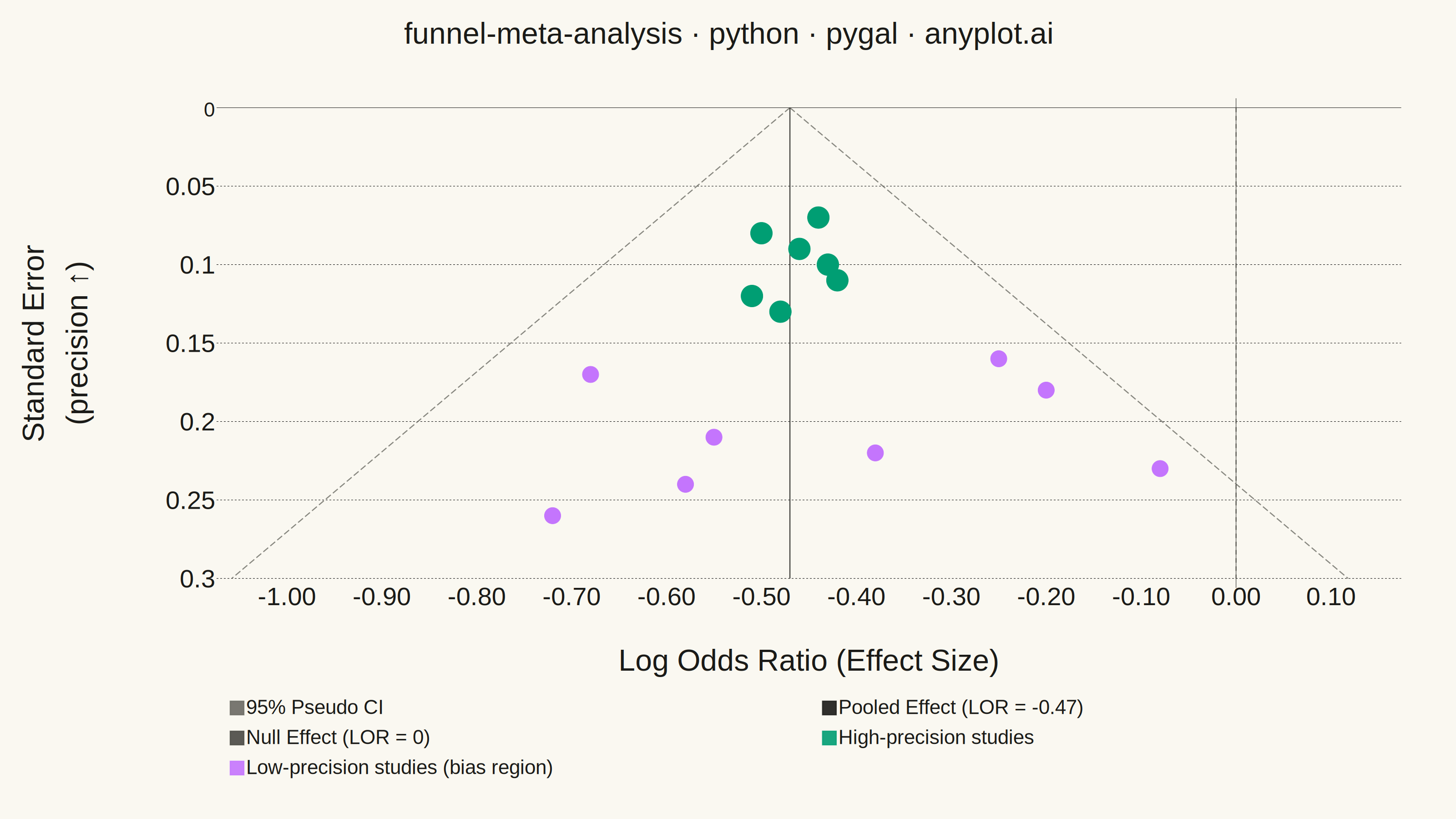
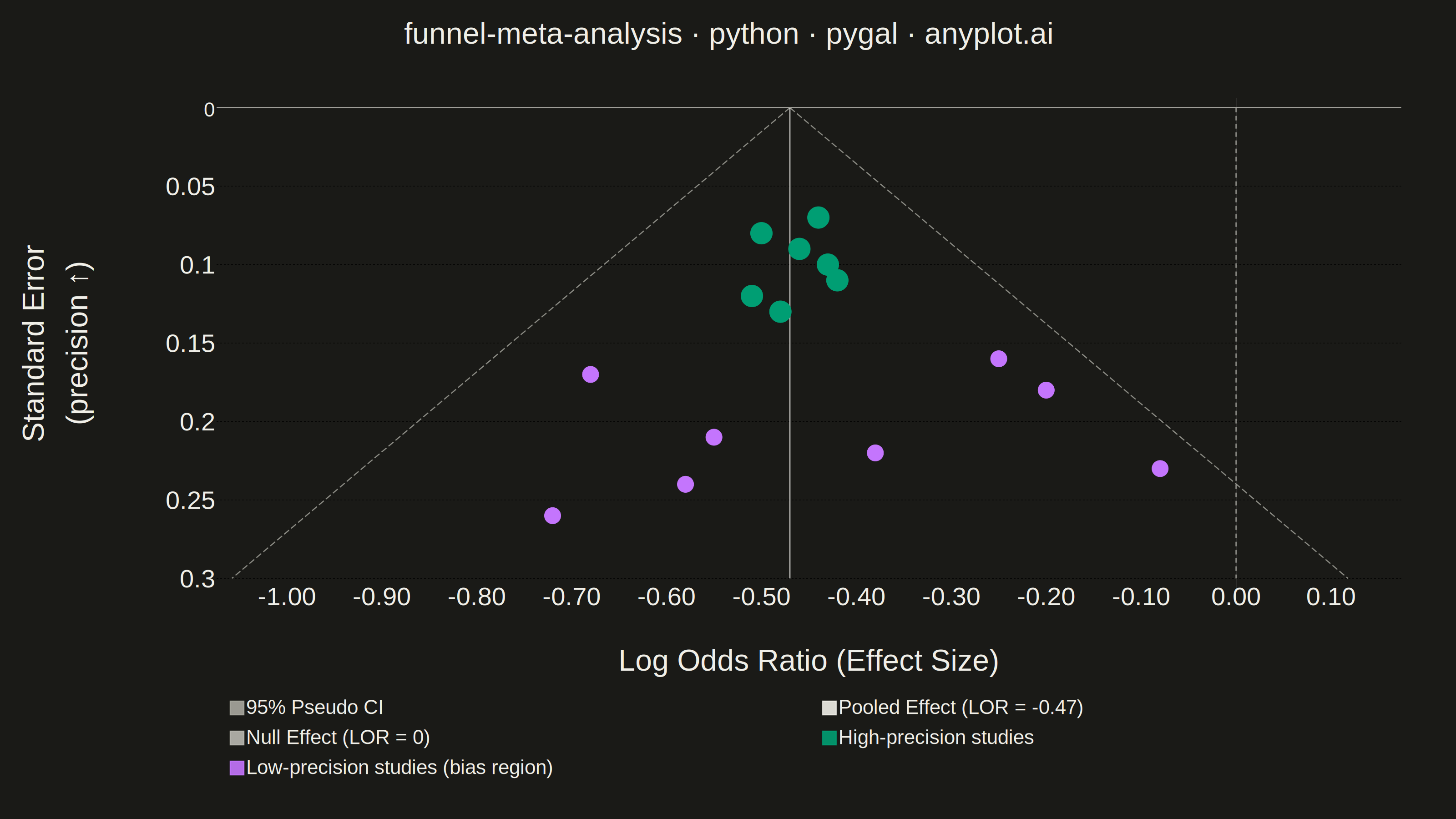
A funnel plot used in meta-analysis to assess publication bias by plotting individual study effect sizes against their precision (typically standard error). Studies scatter around a summary effect line, with pseudo 95% confidence limits forming an inverted funnel shape. In the absence of bias, studies distribute symmetrically around the summary effect; asymmetry suggests publication bias or systematic heterogeneity. This is a standard tool in systematic reviews and Cochrane-style meta-analyses.
""" anyplot.ai
funnel-meta-analysis: Meta-Analysis Funnel Plot for Publication Bias
Library: pygal 3.1.0 | Python 3.13.13
Quality: 88/100 | Updated: 2026-06-10
"""

import os

import numpy as np
import pygal
from pygal.style import Style


# Theme tokens
THEME = os.getenv("ANYPLOT_THEME", "light")
PAGE_BG = "#FAF8F1" if THEME == "light" else "#1A1A17"
INK = "#1A1A17" if THEME == "light" else "#F0EFE8"
INK_SOFT = "#4A4A44" if THEME == "light" else "#B8B7B0"
INK_MUTED = "#6B6A63" if THEME == "light" else "#A8A79F"

# Imprint palette — first categorical series always #009E73
IMPRINT_GREEN = "#009E73"  # position 1 — high-precision studies
IMPRINT_LAVENDER = "#C475FD"  # position 2 — low-precision studies

# Data: 15 RCTs comparing drug vs placebo (log odds ratios)
np.random.seed(42)
study_names = [
    "Adams 2018",
    "Baker 2019",
    "Chen 2019",
    "Davis 2020",
    "Evans 2020",
    "Foster 2021",
    "Garcia 2021",
    "Harris 2022",
    "Ibrahim 2022",
    "Jones 2022",
    "Kim 2023",
    "Lee 2023",
    "Martinez 2023",
    "Nelson 2024",
    "O'Brien 2024",
]

# Effect sizes (log odds ratios) and standard errors
# High-precision studies cluster near pooled effect; low-precision studies
# show rightward asymmetry (missing negative small studies = publication bias)
effect_sizes = np.array(
    [-0.50, -0.42, -0.68, -0.46, -0.25, -0.55, -0.48, -0.44, -0.38, -0.20, -0.72, -0.43, -0.08, -0.51, -0.58]
)
std_errors = np.array([0.08, 0.11, 0.17, 0.09, 0.16, 0.21, 0.13, 0.07, 0.22, 0.18, 0.26, 0.10, 0.23, 0.12, 0.24])

pooled_effect = -0.47

high_precision_mask = std_errors < 0.15
low_precision_mask = ~high_precision_mask

# Style — theme-adaptive chrome + Imprint palette
# Structural reference lines (CI, pooled effect, null) use INK tokens;
# data series (study groups) use Imprint categorical positions 1 and 3.
custom_style = Style(
    background=PAGE_BG,
    plot_background=PAGE_BG,
    foreground=INK,
    foreground_strong=INK,
    foreground_subtle=INK_MUTED,
    colors=(
        INK_MUTED,  # 0: CI left boundary (structural line, not a data category)
        INK_MUTED,  # 1: CI right boundary (hidden from legend)
        INK,  # 2: Pooled effect line (structural reference)
        INK_SOFT,  # 3: Null effect line (structural reference)
        IMPRINT_GREEN,  # 4: High-precision studies — Imprint position 1
        IMPRINT_LAVENDER,  # 5: Low-precision studies — Imprint position 2
    ),
    title_font_size=66,
    label_font_size=56,
    major_label_font_size=44,
    legend_font_size=44,
    value_font_size=36,
    stroke_width=2.5,
    font_family="Helvetica, Arial, sans-serif",
    opacity=".9",
    opacity_hover="1",
)

# Chart — 3200×1800 landscape canvas
chart = pygal.XY(
    width=3200,
    height=1800,
    explicit_size=True,
    title="funnel-meta-analysis · python · pygal · anyplot.ai",
    x_title="Log Odds Ratio (Effect Size)",
    y_title="Standard Error (precision ↑)",
    style=custom_style,
    show_legend=True,
    legend_at_bottom=True,
    legend_at_bottom_columns=2,
    legend_box_size=30,
    dots_size=14,
    stroke=False,
    show_y_guides=True,
    show_x_guides=False,
    margin=120,
    inverse_y_axis=True,
    truncate_legend=-1,
    x_value_formatter=lambda x: f"{x:.2f}",
    y_value_formatter=lambda y: f"{y:.2f}",
    y_labels=[0.00, 0.05, 0.10, 0.15, 0.20, 0.25, 0.30],
    print_values=False,
    print_zeroes=False,
    range=(0, 0.30),
    xrange=(-1.05, 0.15),
    spacing=30,
    tooltip_border_radius=8,
)

# Funnel boundaries — pseudo 95% CI diagonal lines
se_values = np.linspace(0, 0.30, 60)
funnel_left = [(float(pooled_effect - 1.96 * se), float(se)) for se in se_values]
chart.add(
    "95% Pseudo CI",
    funnel_left,
    stroke=True,
    show_dots=False,
    stroke_style={"width": 4, "dasharray": "14, 6"},
    formatter=lambda x: "",
)

funnel_right = [(float(pooled_effect + 1.96 * se), float(se)) for se in se_values]
chart.add(
    None,
    funnel_right,
    stroke=True,
    show_dots=False,
    stroke_style={"width": 4, "dasharray": "14, 6"},
    formatter=lambda x: "",
)

# Vertical line at pooled effect (solid, prominent)
chart.add(
    f"Pooled Effect (LOR = {pooled_effect:.2f})",
    [(float(pooled_effect), 0.0), (float(pooled_effect), 0.30)],
    stroke=True,
    show_dots=False,
    stroke_style={"width": 6},
    formatter=lambda x: "",
)

# Vertical dashed line at null effect
chart.add(
    "Null Effect (LOR = 0)",
    [(0.0, 0.0), (0.0, 0.30)],
    stroke=True,
    show_dots=False,
    stroke_style={"width": 3, "dasharray": "10, 8"},
    formatter=lambda x: "",
)

# High-precision studies — larger markers, tightly clustered near pooled effect
hp_points = [
    {"value": (float(es), float(se)), "label": f"{name}: LOR={es:.2f}, SE={se:.2f}"}
    for name, es, se in zip(
        np.array(study_names)[high_precision_mask],
        effect_sizes[high_precision_mask],
        std_errors[high_precision_mask],
        strict=True,
    )
]
chart.add("High-precision studies", hp_points, stroke=False, dots_size=24, formatter=lambda x: "")

# Low-precision studies — smaller markers, rightward asymmetry signals publication bias
lp_points = [
    {"value": (float(es), float(se)), "label": f"{name}: LOR={es:.2f}, SE={se:.2f}"}
    for name, es, se in zip(
        np.array(study_names)[low_precision_mask],
        effect_sizes[low_precision_mask],
        std_errors[low_precision_mask],
        strict=True,
    )
]
chart.add("Low-precision studies (bias region)", lp_points, stroke=False, dots_size=18, formatter=lambda x: "")

# Save
chart.render_to_png(f"plot-{THEME}.png")
with open(f"plot-{THEME}.html", "wb") as f:
    f.write(chart.render())
Runnable source as JSON, for any HTTP client: https://api.anyplot.ai/specs/funnel-meta-analysis/pygal/code. Any spec id and library id listed in llms-full.txt fit the same URL shape; every URL below is complete and callable.
{
  "spec_id": "funnel-meta-analysis",
  "language": "python",
  "library": "pygal",
  "page": "https://anyplot.ai/funnel-meta-analysis/python/pygal",
  "hub": "https://anyplot.ai/funnel-meta-analysis",
  "code_json": "https://api.anyplot.ai/specs/funnel-meta-analysis/pygal/code",
  "spec_json": "https://api.anyplot.ai/specs/funnel-meta-analysis",
  "render_light_png": "https://storage.googleapis.com/anyplot-images/plots/funnel-meta-analysis/python/pygal/plot-light.png",
  "render_dark_png": "https://storage.googleapis.com/anyplot-images/plots/funnel-meta-analysis/python/pygal/plot-dark.png",
  "interactive_light_html": "https://storage.googleapis.com/anyplot-images/plots/funnel-meta-analysis/python/pygal/plot-light.html",
  "interactive_dark_html": "https://storage.googleapis.com/anyplot-images/plots/funnel-meta-analysis/python/pygal/plot-dark.html",
  "quality_score": 88.0,
  "license": "MIT",
  "guide": "https://anyplot.ai/llms.txt"
}
Part of Meta-Analysis Funnel Plot for Publication Bias on anyplot.ai.