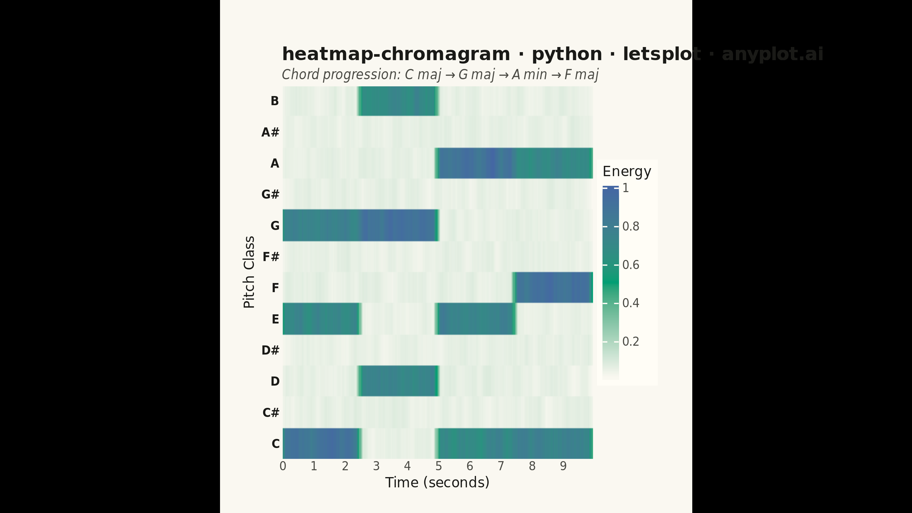
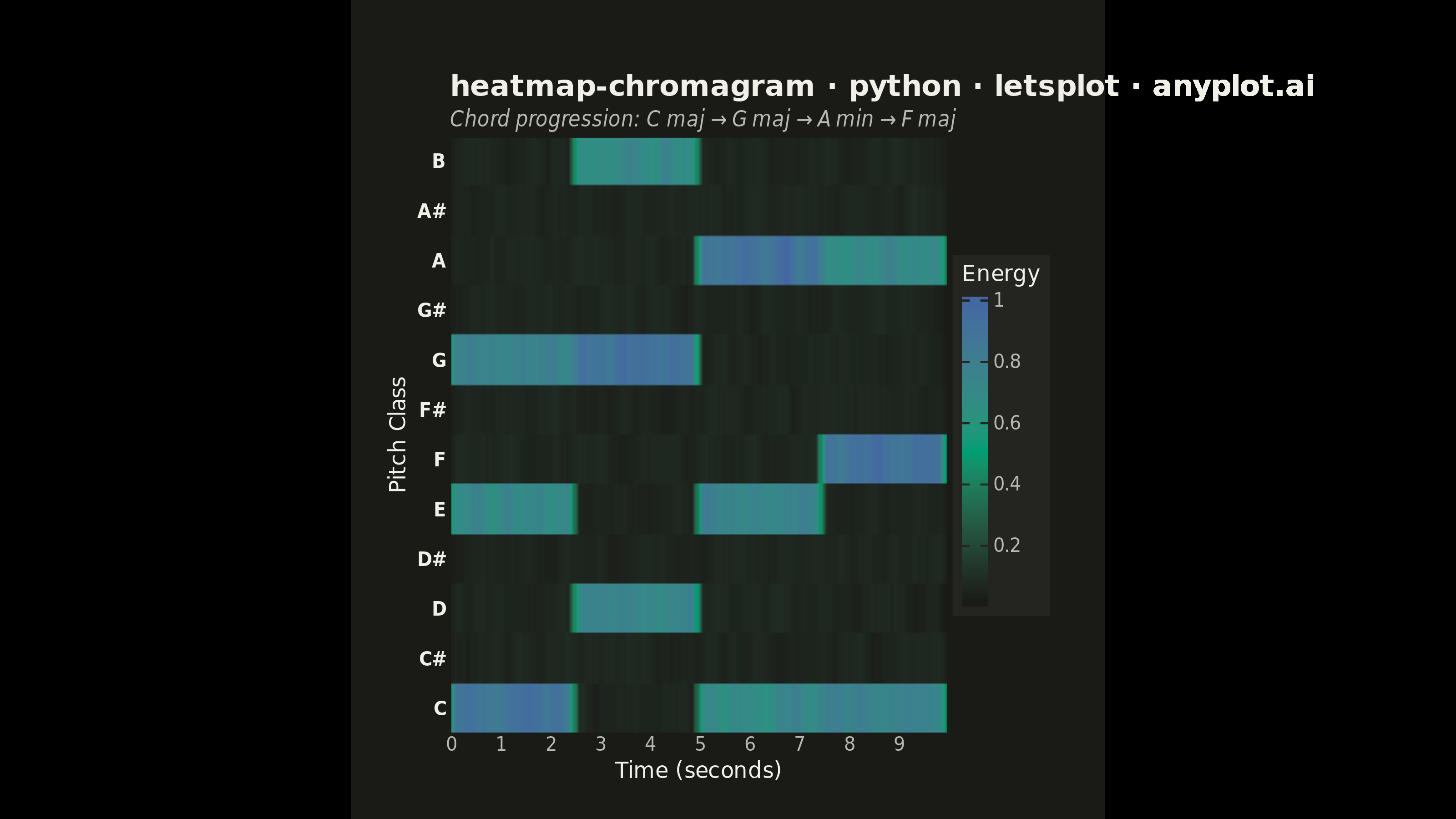
A heatmap-style visualization showing the energy distribution across the 12 pitch classes (C, C#, D, D#, E, F, F#, G, G#, A, A#, B) over time. Each column represents a time frame and each row a pitch class, with color intensity indicating the energy or magnitude at that pitch-time point. Widely used in music information retrieval to analyze harmonic content, detect chords, estimate musical key, and study tonal progressions in audio signals.
""" anyplot.ai
heatmap-chromagram: Music Chromagram (Pitch Class Distribution over Time)
Library: letsplot 4.10.1 | Python 3.13.14
Quality: 84/100 | Updated: 2026-06-24
"""

import os

import numpy as np
import pandas as pd
from lets_plot import (
    LetsPlot,
    aes,
    element_blank,
    element_rect,
    element_text,
    geom_raster,
    ggplot,
    ggsize,
    guide_colorbar,
    labs,
    layer_tooltips,
    scale_fill_gradientn,
    scale_x_continuous,
    scale_y_continuous,
    theme,
)
from lets_plot.export import ggsave
from PIL import Image, ImageDraw


LetsPlot.setup_html()

# Theme tokens — Imprint palette, theme-adaptive chrome
THEME = os.getenv("ANYPLOT_THEME", "light")
PAGE_BG = "#FAF8F1" if THEME == "light" else "#1A1A17"
ELEVATED_BG = "#FFFDF6" if THEME == "light" else "#242420"
INK = "#1A1A17" if THEME == "light" else "#F0EFE8"
INK_SOFT = "#4A4A44" if THEME == "light" else "#B8B7B0"


def _fix_canvas_margin(path, bg_color):
    """Replace letsplot's white outer canvas margin with bg_color via edge flood-fill."""
    img = Image.open(path).convert("RGB")
    w, h = img.size
    bg_tuple = tuple(int(bg_color[i : i + 2], 16) for i in (1, 3, 5))
    for corner in [(0, 0), (w - 1, 0), (0, h - 1), (w - 1, h - 1)]:
        if all(c >= 245 for c in img.getpixel(corner)):
            ImageDraw.floodfill(img, corner, bg_tuple, thresh=10)
    img.save(path)


# Imprint sequential gradient: background → brand green → blue (single-polarity energy)
SEQ_COLORS = [PAGE_BG, "#009E73", "#4467A3"]

# Data — synthetic chromagram: C major → G major → A minor → F major
np.random.seed(42)
pitch_classes = ["C", "C#", "D", "D#", "E", "F", "F#", "G", "G#", "A", "A#", "B"]
n_pitches = len(pitch_classes)
n_frames = 200
frame_duration = 0.05
time_seconds = np.arange(n_frames) * frame_duration

chroma = np.random.uniform(0.02, 0.10, (n_pitches, n_frames))

chords = {
    "C_major": [0, 4, 7],  # C, E, G
    "G_major": [7, 11, 2],  # G, B, D
    "A_minor": [9, 0, 4],  # A, C, E
    "F_major": [5, 9, 0],  # F, A, C
}

segments = [(0, 50, "C_major"), (50, 100, "G_major"), (100, 150, "A_minor"), (150, 200, "F_major")]

for start, end, chord_name in segments:
    root, third, fifth = chords[chord_name]
    chroma[root, start:end] += np.random.uniform(0.7, 0.95, end - start)
    chroma[third, start:end] += np.random.uniform(0.5, 0.75, end - start)
    chroma[fifth, start:end] += np.random.uniform(0.55, 0.8, end - start)

kernel = np.ones(5) / 5
for i in range(n_pitches):
    chroma[i] = np.convolve(chroma[i], kernel, mode="same")

chroma = chroma / chroma.max()

time_grid, pitch_grid = np.meshgrid(time_seconds, np.arange(n_pitches))
df = pd.DataFrame(
    {
        "time": time_grid.ravel(),
        "pitch_idx": pitch_grid.ravel(),
        "energy": np.round(chroma.ravel(), 4),
        "pitch_name": np.repeat(pitch_classes, n_frames),
    }
)

# Title with length-aware font size scaling
title = "heatmap-chromagram · python · letsplot · anyplot.ai"
title_fontsize = round(16 * (67 / len(title))) if len(title) > 67 else 16

# Plot
plot = (
    ggplot(df, aes(x="time", y="pitch_idx", fill="energy"))
    + geom_raster(
        tooltips=layer_tooltips()
        .format("@time", ".2f")
        .format("@energy", ".3f")
        .line("@pitch_name at @time s")
        .line("Energy: @energy")
    )
    + scale_fill_gradientn(colors=SEQ_COLORS, name="Energy", guide=guide_colorbar(barwidth=14, barheight=170, nbin=256))
    + scale_x_continuous(
        name="Time (seconds)", breaks=list(np.arange(0, n_frames * frame_duration + 0.5, 1.0)), expand=[0, 0]
    )
    + scale_y_continuous(name="Pitch Class", breaks=list(range(n_pitches)), labels=pitch_classes, expand=[0, 0])
    + labs(title=title, subtitle="Chord progression: C maj → G maj → A min → F maj")
    + theme(
        plot_title=element_text(size=title_fontsize, face="bold", color=INK),
        plot_subtitle=element_text(size=12, color=INK_SOFT, face="italic"),
        axis_title_x=element_text(size=12, color=INK),
        axis_title_y=element_text(size=12, color=INK),
        axis_text_x=element_text(size=10, color=INK_SOFT),
        axis_text_y=element_text(size=10, face="bold", color=INK),
        axis_ticks=element_blank(),
        axis_line=element_blank(),
        legend_text=element_text(size=10, color=INK_SOFT),
        legend_title=element_text(size=12, color=INK),
        panel_grid=element_blank(),
        panel_background=element_rect(fill=PAGE_BG, color=PAGE_BG),
        plot_background=element_rect(fill=PAGE_BG, color=PAGE_BG),
        plot_margin=[40, 30, 20, 20],
        legend_background=element_rect(fill=ELEVATED_BG, color=INK_SOFT),
    )
    + ggsize(800, 450)
)

# Save — scale=4 produces 3200×1800 px from ggsize(800, 450)
ggsave(plot, f"plot-{THEME}.png", path=".", scale=4)
_fix_canvas_margin(f"plot-{THEME}.png", PAGE_BG)
ggsave(plot, f"plot-{THEME}.html", path=".")
Runnable source as JSON, for any HTTP client: https://api.anyplot.ai/specs/heatmap-chromagram/letsplot/code. Any spec id and library id listed in llms-full.txt fit the same URL shape; every URL below is complete and callable.
{
  "spec_id": "heatmap-chromagram",
  "language": "python",
  "library": "letsplot",
  "page": "https://anyplot.ai/heatmap-chromagram/python/letsplot",
  "hub": "https://anyplot.ai/heatmap-chromagram",
  "code_json": "https://api.anyplot.ai/specs/heatmap-chromagram/letsplot/code",
  "spec_json": "https://api.anyplot.ai/specs/heatmap-chromagram",
  "render_light_png": "https://storage.googleapis.com/anyplot-images/plots/heatmap-chromagram/python/letsplot/plot-light.png",
  "render_dark_png": "https://storage.googleapis.com/anyplot-images/plots/heatmap-chromagram/python/letsplot/plot-dark.png",
  "interactive_light_html": "https://storage.googleapis.com/anyplot-images/plots/heatmap-chromagram/python/letsplot/plot-light.html",
  "interactive_dark_html": "https://storage.googleapis.com/anyplot-images/plots/heatmap-chromagram/python/letsplot/plot-dark.html",
  "quality_score": 84.0,
  "license": "MIT",
  "guide": "https://anyplot.ai/llms.txt"
}
Part of Music Chromagram (Pitch Class Distribution over Time) on anyplot.ai.