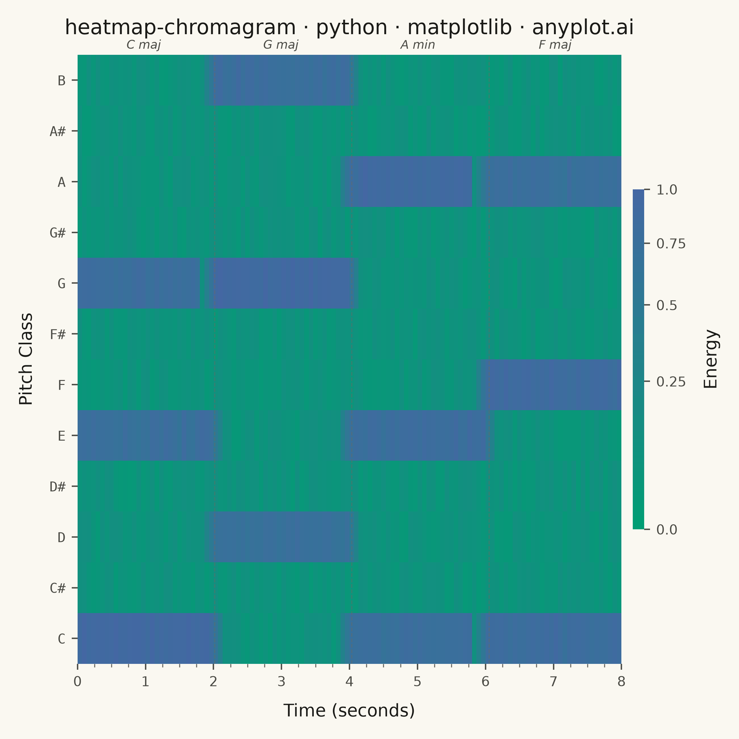
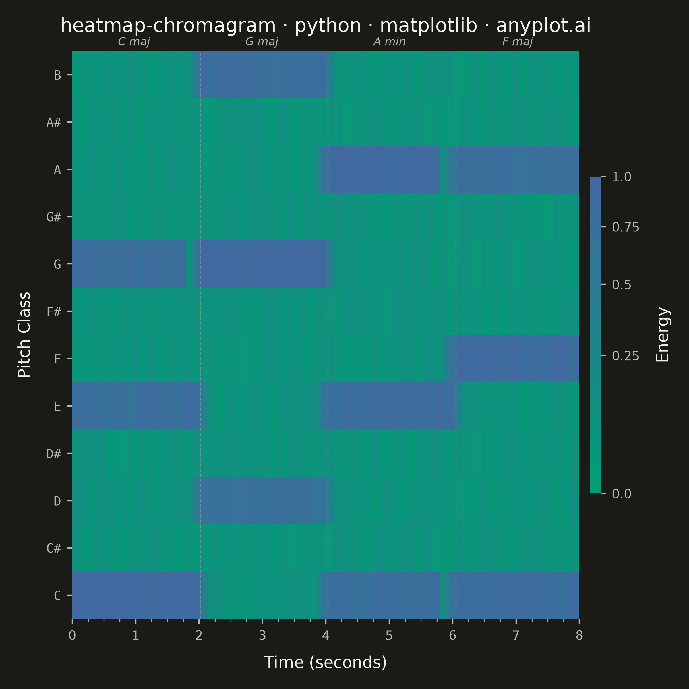
Music Chromagram (Pitch Class Distribution over Time) — Matplotlib

A heatmap-style visualization showing the energy distribution across the 12 pitch classes (C, C#, D, D#, E, F, F#, G, G#, A, A#, B) over time. Each column represents a time frame and each row a pitch class, with color intensity indicating the energy or magnitude at that pitch-time point. Widely used in music information retrieval to analyze harmonic content, detect chords, estimate musical key, and study tonal progressions in audio signals.

Music Chromagram (Pitch Class Distribution over Time) rendered with Matplotlib

Python source (Matplotlib)

""" anyplot.ai
heatmap-chromagram: Music Chromagram (Pitch Class Distribution over Time)
Library: matplotlib 3.11.0 | Python 3.13.14
Quality: 93/100 | Updated: 2026-06-24
"""

import os

import matplotlib.colors as mcolors
import matplotlib.pyplot as plt
import matplotlib.ticker as mticker
import numpy as np


# Theme-adaptive chrome
THEME = os.getenv("ANYPLOT_THEME", "light")
PAGE_BG = "#FAF8F1" if THEME == "light" else "#1A1A17"
ELEVATED_BG = "#FFFDF6" if THEME == "light" else "#242420"
INK = "#1A1A17" if THEME == "light" else "#F0EFE8"
INK_SOFT = "#4A4A44" if THEME == "light" else "#B8B7B0"
INK_MUTED = "#6B6A63" if THEME == "light" else "#A8A79F"

# Imprint sequential colormap (green → blue) for single-polarity energy heatmap
imprint_seq = mcolors.LinearSegmentedColormap.from_list("imprint_seq", ["#009E73", "#4467A3"])

# Data — simulate a chromagram for a short musical passage
# Classic I-V-vi-IV pop chord progression over 8 seconds
np.random.seed(42)

pitch_classes = ["C", "C#", "D", "D#", "E", "F", "F#", "G", "G#", "A", "A#", "B"]
n_pitches = len(pitch_classes)
n_frames = 120
time_seconds = np.linspace(0, 8, n_frames)

# Low background energy across all pitches
chroma = np.random.uniform(0.02, 0.12, (n_pitches, n_frames))

# Chord regions with realistic harmonic energy
chord_regions = [
    (0, 30, "C maj", {"C": 0.9, "E": 0.75, "G": 0.8}),
    (30, 60, "G maj", {"G": 0.92, "B": 0.78, "D": 0.72}),
    (60, 90, "A min", {"A": 0.88, "C": 0.76, "E": 0.82}),
    (90, 120, "F maj", {"F": 0.85, "A": 0.74, "C": 0.80}),
]

for start, end, _, notes in chord_regions:
    for note, energy in notes.items():
        idx = pitch_classes.index(note)
        chroma[idx, start:end] = energy + np.random.normal(0, 0.05, end - start)
        # Harmonic bleeding at chord boundaries for realism
        if start > 0:
            chroma[idx, start - 3 : start] = np.linspace(0.1, energy * 0.7, 3)
        if end < n_frames:
            tail = min(3, n_frames - end)
            chroma[idx, end : end + tail] = np.linspace(energy * 0.7, 0.1, tail)

chroma = np.clip(chroma, 0, 1)

# PowerNorm enhances perceptual contrast between quiet and active pitch regions
norm = mcolors.PowerNorm(gamma=0.6, vmin=0, vmax=1)

# Canvas — square (2400×2400) for symmetric heatmap
fig, ax = plt.subplots(figsize=(6, 6), dpi=400, facecolor=PAGE_BG)
ax.set_facecolor(PAGE_BG)

time_edges = np.linspace(0, 8, n_frames + 1)
pitch_edges = np.arange(n_pitches + 1) - 0.5

im = ax.pcolormesh(time_edges, pitch_edges, chroma, cmap=imprint_seq, norm=norm, shading="flat", rasterized=True)

# Chord region labels and subtle dividers for harmonic storytelling
for start, end, label, _ in chord_regions:
    t_mid = (time_seconds[start] + time_seconds[min(end - 1, n_frames - 1)]) / 2
    ax.text(
        t_mid,
        n_pitches - 0.2,
        label,
        ha="center",
        va="top",
        fontsize=7,
        fontstyle="italic",
        color=INK_SOFT,
        fontweight="medium",
    )
    if start > 0:
        t_boundary = time_seconds[start]
        ax.axvline(t_boundary, color=INK_MUTED, linewidth=0.6, linestyle="--", alpha=0.5)

# Axes
ax.set_yticks(np.arange(n_pitches))
ax.set_yticklabels(pitch_classes, fontsize=8, fontfamily="monospace", color=INK_SOFT)
ax.set_xlabel("Time (seconds)", fontsize=10, color=INK, labelpad=8)
ax.set_ylabel("Pitch Class", fontsize=10, color=INK, labelpad=8)

title = "heatmap-chromagram · python · matplotlib · anyplot.ai"
title_fontsize = max(8, round(12 * 67 / len(title))) if len(title) > 67 else 12
ax.set_title(title, fontsize=title_fontsize, fontweight="medium", color=INK, pad=12)

ax.tick_params(axis="both", labelsize=8, colors=INK_SOFT, labelcolor=INK_SOFT)
ax.xaxis.set_major_locator(mticker.MultipleLocator(1))
ax.xaxis.set_minor_locator(mticker.MultipleLocator(0.25))
ax.tick_params(axis="x", which="minor", length=2, color=INK_MUTED)

for spine in ax.spines.values():
    spine.set_visible(False)

# Colorbar with theme-adaptive styling
cbar = fig.colorbar(im, ax=ax, fraction=0.02, pad=0.02, aspect=30)
cbar.set_label("Energy", fontsize=10, labelpad=10, color=INK)
cbar.ax.tick_params(labelsize=8, colors=INK_SOFT, labelcolor=INK_SOFT)
cbar.outline.set_visible(False)
cbar.set_ticks([0, 0.25, 0.5, 0.75, 1.0])
cbar.ax.set_yticklabels(["0.0", "0.25", "0.5", "0.75", "1.0"], color=INK_SOFT, fontsize=8)

plt.tight_layout()
plt.savefig(f"plot-{THEME}.png", dpi=400, facecolor=PAGE_BG)
plt.close()

Part of Music Chromagram (Pitch Class Distribution over Time) on anyplot.ai.

Music Chromagram (Pitch Class Distribution over Time) — Matplotlib

Python source (Matplotlib)

Other implementations