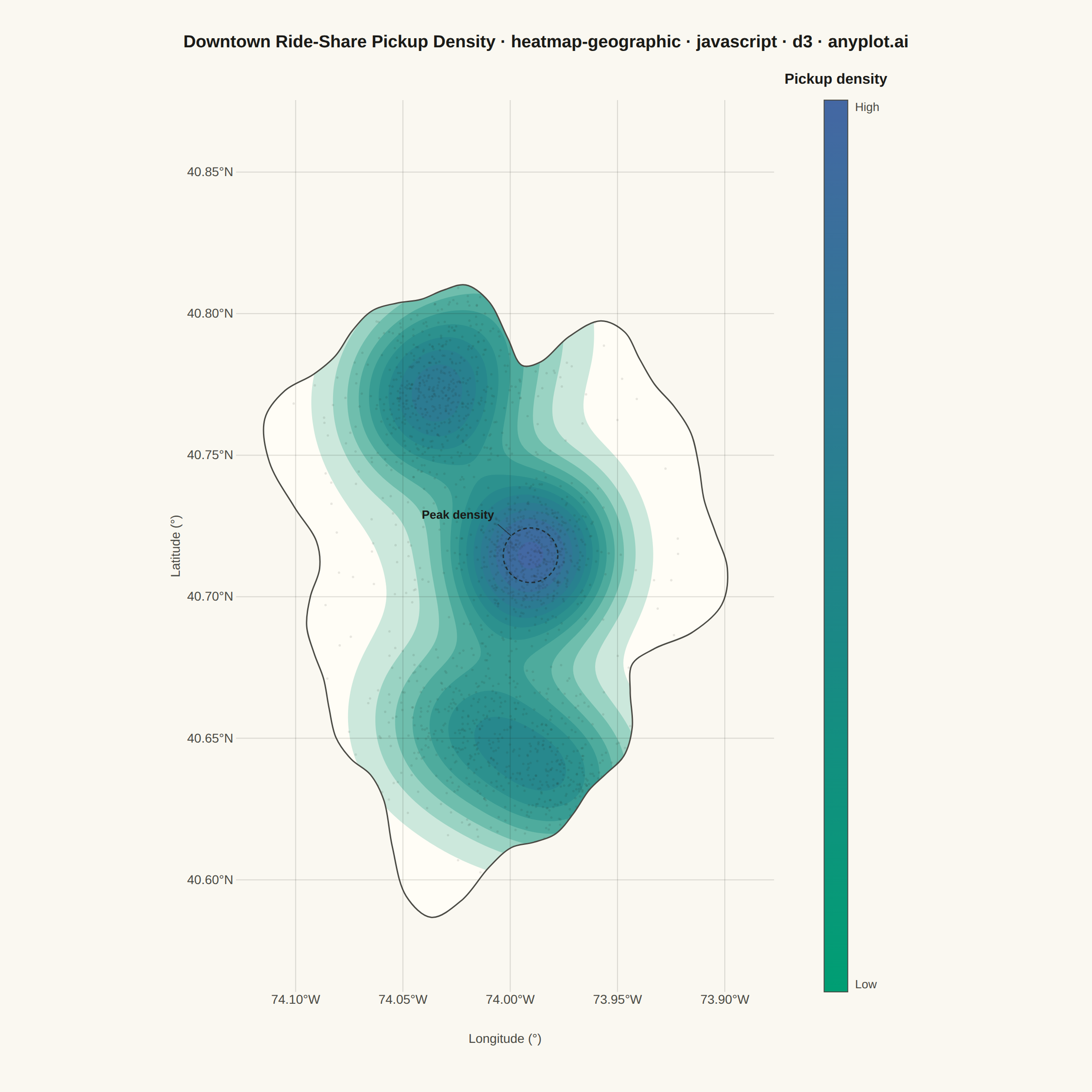
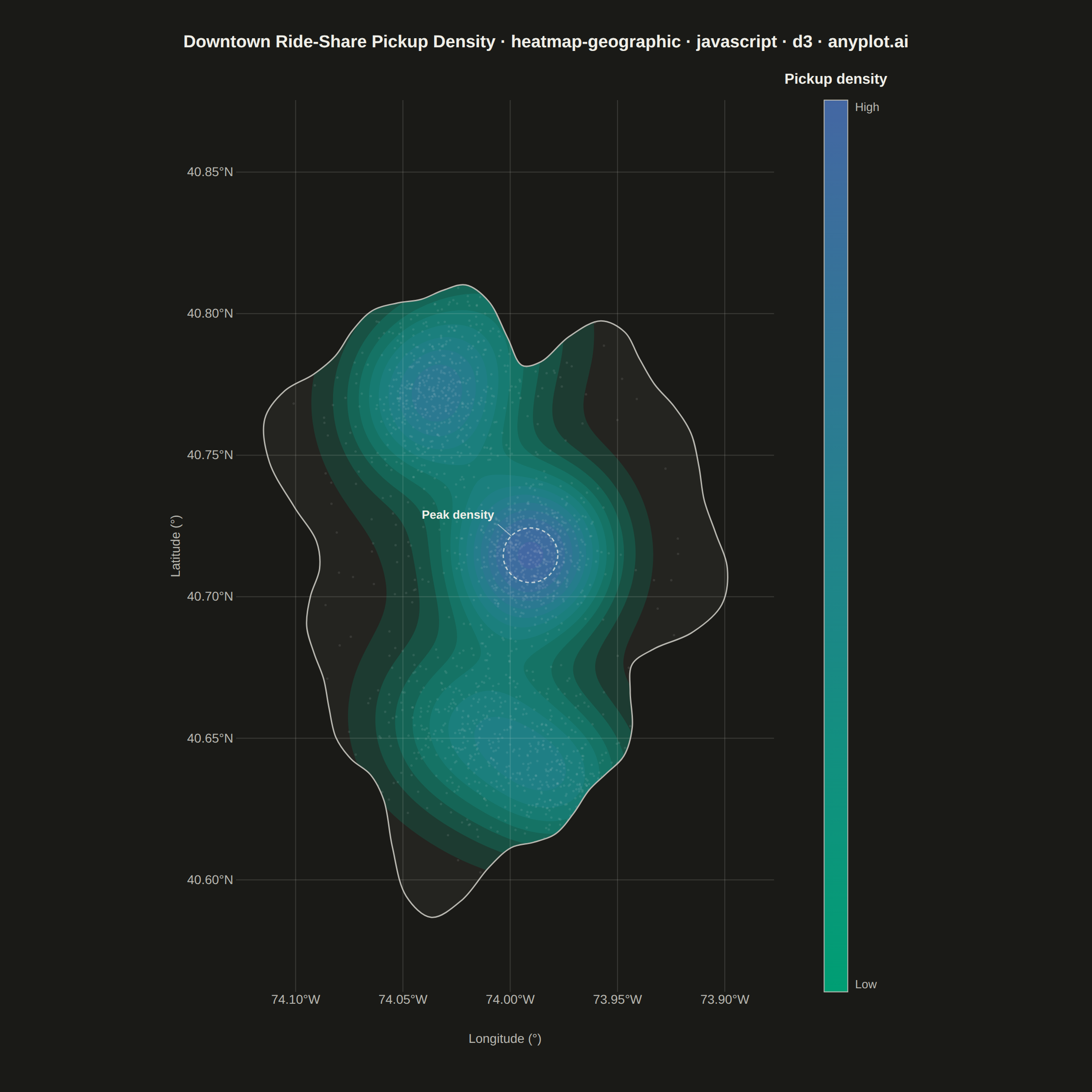
The same plot in 14 other libraries — JavaScript: Chart.js, Apache ECharts, Highcharts, MUI X Charts; Python: Altair, Bokeh, lets-plot, Matplotlib, Plotly, plotnine, Pygal, Seaborn; R: ggplot2; Julia: Makie.jl. Compare all 15 side by side: Geographic Heatmap for Spatial Density in Python, R, Julia and JavaScript.
A geographic heatmap visualizes spatial density or intensity values across a map using continuous color gradients. Unlike choropleth maps that color discrete regions, this plot shows smooth density variations computed from point data or gridded values. The color intensity at each location represents the concentration or magnitude of the underlying data, making it ideal for identifying hotspots, clusters, and spatial patterns in geographic data.
// anyplot.ai
// heatmap-geographic: Geographic Heatmap for Spatial Density
// Library: d3 7.9.0 | JavaScript 22.23.2
// Quality: 94/100 | Created: 2026-09-02

//# anyplot-orientation: square
const t = window.ANYPLOT_TOKENS;
const { width, height } = window.ANYPLOT_SIZE;

// --- Deterministic PRNG (browser has no seeded Math.random) -----------------
let seed = 42;
function rand() {
  seed = (seed * 1103515245 + 12345) & 0x7fffffff;
  return seed / 0x7fffffff;
}
function gaussianJitter(sigma) {
  const u1 = Math.max(rand(), 1e-6);
  const u2 = rand();
  return sigma * Math.sqrt(-2 * Math.log(u1)) * Math.cos(2 * Math.PI * u2);
}

// --- Basemap: stylized coastal-district outline (illustrative, not a survey) -
const centerLon = -74.01; // Downtown Manhattan / Financial District
const centerLat = 40.71;
const halfLonDeg = 0.095;
const halfLatDeg = 0.1;
const coastPoints = 56;
const coastline = d3.range(coastPoints).map((i) => {
  const theta = (i / coastPoints) * 2 * Math.PI;
  const r =
    1 +
    0.14 * Math.sin(3 * theta + 0.6) +
    0.08 * Math.sin(7 * theta + 1.7) +
    0.05 * Math.sin(11 * theta + 2.9);
  return [centerLon + halfLonDeg * r * Math.cos(theta), centerLat + halfLatDeg * r * Math.sin(theta)];
});

// --- Data: ride-share pickup locations, clustered around activity hubs ------
const hotspots = [
  { lon: centerLon - 0.028, lat: centerLat + 0.06, count: 420, sigma: 0.016 }, // north business district
  { lon: centerLon + 0.02, lat: centerLat + 0.005, count: 520, sigma: 0.013 }, // central transit hub
  { lon: centerLon - 0.008, lat: centerLat - 0.055, count: 300, sigma: 0.018 }, // south waterfront
  { lon: centerLon + 0.032, lat: centerLat - 0.075, count: 260, sigma: 0.014 }, // south tip nightlife
  { lon: centerLon + 0.004, lat: centerLat + 0.09, count: 180, sigma: 0.019 }, // north residential node
];

const pickups = [];
for (const h of hotspots) {
  for (let i = 0; i < h.count; i += 1) {
    pickups.push({
      lon: h.lon + gaussianJitter(h.sigma),
      lat: h.lat + gaussianJitter(h.sigma * 0.85),
    });
  }
}
for (let i = 0; i < 220; i += 1) {
  pickups.push({
    lon: centerLon + gaussianJitter(halfLonDeg * 0.5),
    lat: centerLat + gaussianJitter(halfLatDeg * 0.5),
  });
}

// --- Layout -------------------------------------------------------------
const margin = { top: 110, right: 200, bottom: 110, left: 110 };
const mapAreaW = width - margin.left - margin.right;
const mapAreaH = height - margin.top - margin.bottom;

const lonValues = coastline.map((d) => d[0]).concat(pickups.map((d) => d.lon));
const latValues = coastline.map((d) => d[1]).concat(pickups.map((d) => d.lat));
const [lonMin0, lonMax0] = d3.extent(lonValues);
const [latMin0, latMax0] = d3.extent(latValues);
const lonPad = (lonMax0 - lonMin0) * 0.06;
const latPad = (latMax0 - latMin0) * 0.06;
const lonExtent = [lonMin0 - lonPad, lonMax0 + lonPad];
const latExtent = [latMin0 - latPad, latMax0 + latPad];

const lonSpan = lonExtent[1] - lonExtent[0];
const latSpan = latExtent[1] - latExtent[0];
const effectiveLonSpan = lonSpan * Math.cos((centerLat * Math.PI) / 180);
const dataAspect = latSpan / effectiveLonSpan; // height / width, true-distance corrected

let mapW;
let mapH;
if (dataAspect > mapAreaH / mapAreaW) {
  mapH = mapAreaH;
  mapW = mapH / dataAspect;
} else {
  mapW = mapAreaW;
  mapH = mapW * dataAspect;
}
const offsetX = margin.left + (mapAreaW - mapW) / 2;
const offsetY = margin.top + (mapAreaH - mapH) / 2;

const xScale = d3.scaleLinear().domain(lonExtent).range([offsetX, offsetX + mapW]);
const yScale = d3.scaleLinear().domain(latExtent).range([offsetY + mapH, offsetY]);

// --- Kernel density estimate over the pickup points -------------------------
const density = d3
  .contourDensity()
  .x((d) => xScale(d.lon))
  .y((d) => yScale(d.lat))
  .size([width, height])
  .bandwidth(45)
  .thresholds(12)(pickups);

const maxDensity = Math.max(d3.max(density, (d) => d.value), 1e-6);
const densityColor = (v) => d3.interpolateRgbBasis(t.seq)(Math.min(v / maxDensity, 1));

// --- SVG mount ----------------------------------------------------------
const svg = d3.select("#container").append("svg").attr("width", width).attr("height", height);

const lineGen = d3
  .line()
  .x((d) => xScale(d[0]))
  .y((d) => yScale(d[1]))
  .curve(d3.curveCatmullRomClosed.alpha(0.5));
const landD = lineGen(coastline);

svg.append("defs").append("clipPath").attr("id", "landClip").append("path").attr("d", landD);

// map-layer: everything that pans/scales together under d3.zoom()
const mapLayer = svg.append("g").attr("class", "map-layer");

// land base
mapLayer.append("path").attr("d", landD).attr("fill", t.elevatedBg);

// density contours + point texture, clipped to the landmass
const clipped = mapLayer.append("g").attr("clip-path", "url(#landClip)");
clipped
  .selectAll("path.contour")
  .data(density)
  .join("path")
  .attr("class", "contour")
  .attr("d", d3.geoPath())
  .attr("fill", (d) => densityColor(d.value))
  .attr("fill-opacity", (d) => 0.15 + 0.7 * (d.value / maxDensity))
  .attr("stroke", "none");

clipped
  .selectAll("circle")
  .data(pickups)
  .join("circle")
  .attr("cx", (d) => xScale(d.lon))
  .attr("cy", (d) => yScale(d.lat))
  .attr("r", 1.3)
  .attr("fill", t.ink)
  .attr("opacity", 0.1);

// coastline outline, crisp on top of the fills
mapLayer.append("path").attr("d", landD).attr("fill", "none").attr("stroke", t.inkSoft).attr("stroke-width", 1.5);

// --- Annotation: highlight the single strongest density peak ---------------
const peakContour = density.reduce((a, b) => (b.value > a.value ? b : a));
const [peakX, peakY] = d3.polygonCentroid(peakContour.coordinates[0][0]);
const peakLabelX = peakX - 40;
const peakLabelY = peakY - 40;

const annotation = svg.append("g").attr("class", "peak-annotation");
annotation
  .append("circle")
  .attr("cx", peakX)
  .attr("cy", peakY)
  .attr("r", 30)
  .attr("fill", "none")
  .attr("stroke", t.ink)
  .attr("stroke-width", 1.5)
  .attr("stroke-dasharray", "4,3")
  .attr("opacity", 0.75);
annotation
  .append("line")
  .attr("x1", peakX - 21)
  .attr("y1", peakY - 21)
  .attr("x2", peakLabelX + 4)
  .attr("y2", peakLabelY + 6)
  .attr("stroke", t.ink)
  .attr("stroke-width", 1)
  .attr("opacity", 0.6);
annotation
  .append("text")
  .attr("x", peakLabelX)
  .attr("y", peakLabelY)
  .attr("text-anchor", "end")
  .attr("fill", t.ink)
  .style("font-size", "13px")
  .style("font-weight", "600")
  .text("Peak density");

// --- Axes (lon/lat reference grid) -------------------------------------
const lonFormat = (d) => `${Math.abs(d).toFixed(2)}°${d < 0 ? "W" : "E"}`;
const latFormat = (d) => `${Math.abs(d).toFixed(2)}°${d < 0 ? "S" : "N"}`;

const xAxis = svg
  .append("g")
  .attr("transform", `translate(0,${offsetY + mapH})`)
  .call(d3.axisBottom(xScale).ticks(5).tickFormat(lonFormat).tickSize(-mapH));
const yAxis = svg
  .append("g")
  .attr("transform", `translate(${offsetX},0)`)
  .call(d3.axisLeft(yScale).ticks(5).tickFormat(latFormat).tickSize(-mapW));

for (const axis of [xAxis, yAxis]) {
  axis.selectAll("text").attr("fill", t.inkSoft).style("font-size", "14px");
  axis.selectAll("line").attr("stroke", t.grid);
  axis.select(".domain").remove();
}

svg
  .append("text")
  .attr("x", offsetX + mapW / 2)
  .attr("y", offsetY + mapH + 56)
  .attr("text-anchor", "middle")
  .attr("fill", t.inkSoft)
  .style("font-size", "14px")
  .text("Longitude (°)");

svg
  .append("text")
  .attr("transform", `translate(${offsetX - 62},${offsetY + mapH / 2}) rotate(-90)`)
  .attr("text-anchor", "middle")
  .attr("fill", t.inkSoft)
  .style("font-size", "14px")
  .text("Latitude (°)");

// --- Zoom: pan/scale the map to explore density at different scales --------
const zoom = d3
  .zoom()
  .scaleExtent([1, 6])
  .translateExtent([
    [offsetX, offsetY],
    [offsetX + mapW, offsetY + mapH],
  ])
  .extent([
    [offsetX, offsetY],
    [offsetX + mapW, offsetY + mapH],
  ])
  .on("zoom", (event) => {
    mapLayer.attr("transform", event.transform);
    const zx = event.transform.rescaleX(xScale);
    const zy = event.transform.rescaleY(yScale);
    xAxis.call(d3.axisBottom(zx).ticks(5).tickFormat(lonFormat).tickSize(-mapH));
    yAxis.call(d3.axisLeft(zy).ticks(5).tickFormat(latFormat).tickSize(-mapW));
    for (const axis of [xAxis, yAxis]) {
      axis.selectAll("text").attr("fill", t.inkSoft).style("font-size", "14px");
      axis.selectAll("line").attr("stroke", t.grid);
      axis.select(".domain").remove();
    }
  });

svg.call(zoom);

// --- Legend: density gradient -------------------------------------------
const legendX = offsetX + mapW + 55;
const legendW = 26;

const gradient = svg
  .append("defs")
  .append("linearGradient")
  .attr("id", "imprintSeqGradient")
  .attr("x1", "0%")
  .attr("y1", "100%")
  .attr("x2", "0%")
  .attr("y2", "0%");
gradient
  .selectAll("stop")
  .data(d3.range(0, 1.0001, 0.1))
  .join("stop")
  .attr("offset", (d) => `${d * 100}%`)
  .attr("stop-color", (d) => d3.interpolateRgbBasis(t.seq)(d));

svg
  .append("rect")
  .attr("x", legendX)
  .attr("y", offsetY)
  .attr("width", legendW)
  .attr("height", mapH)
  .attr("fill", "url(#imprintSeqGradient)")
  .attr("stroke", t.inkSoft)
  .attr("stroke-width", 1);

svg
  .append("text")
  .attr("x", legendX + legendW / 2)
  .attr("y", offsetY - 18)
  .attr("text-anchor", "middle")
  .attr("fill", t.ink)
  .style("font-size", "16px")
  .style("font-weight", "600")
  .text("Pickup density");

svg
  .append("text")
  .attr("x", legendX + legendW + 8)
  .attr("y", offsetY + mapH - 4)
  .attr("fill", t.inkSoft)
  .style("font-size", "13px")
  .text("Low");

svg
  .append("text")
  .attr("x", legendX + legendW + 8)
  .attr("y", offsetY + 12)
  .attr("fill", t.inkSoft)
  .style("font-size", "13px")
  .text("High");

// --- Title ---------------------------------------------------------------
const titleText = "Downtown Ride-Share Pickup Density · heatmap-geographic · javascript · d3 · anyplot.ai";
const defaultTitleSize = 24;
const titleSize =
  titleText.length > 67 ? Math.max(16, Math.round((defaultTitleSize * 67) / titleText.length)) : defaultTitleSize;

svg
  .append("text")
  .attr("x", width / 2)
  .attr("y", 52)
  .attr("text-anchor", "middle")
  .attr("fill", t.ink)
  .style("font-size", `${titleSize}px`)
  .style("font-weight", "600")
  .text(titleText);
Runnable source as JSON, for any HTTP client: https://api.anyplot.ai/specs/heatmap-geographic/d3/code. Any spec id and library id listed in llms-full.txt fit the same URL shape; every URL below is complete and callable.
{
  "spec_id": "heatmap-geographic",
  "language": "javascript",
  "library": "d3",
  "page": "https://anyplot.ai/heatmap-geographic/javascript/d3",
  "hub": "https://anyplot.ai/heatmap-geographic",
  "code_json": "https://api.anyplot.ai/specs/heatmap-geographic/d3/code",
  "spec_json": "https://api.anyplot.ai/specs/heatmap-geographic",
  "render_light_png": "https://storage.googleapis.com/anyplot-images/plots/heatmap-geographic/javascript/d3/plot-light.png",
  "render_dark_png": "https://storage.googleapis.com/anyplot-images/plots/heatmap-geographic/javascript/d3/plot-dark.png",
  "interactive_light_html": "https://storage.googleapis.com/anyplot-images/plots/heatmap-geographic/javascript/d3/plot-light.html",
  "interactive_dark_html": "https://storage.googleapis.com/anyplot-images/plots/heatmap-geographic/javascript/d3/plot-dark.html",
  "quality_score": 94.0,
  "license": "MIT",
  "guide": "https://anyplot.ai/llms.txt"
}
Part of Geographic Heatmap for Spatial Density on anyplot.ai.