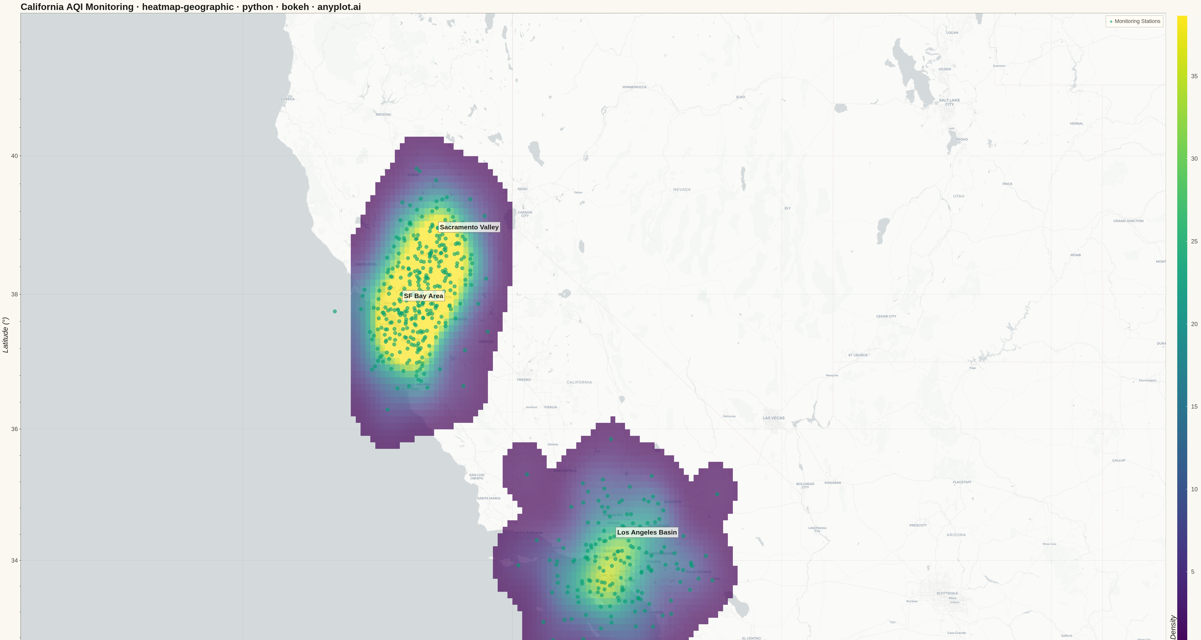
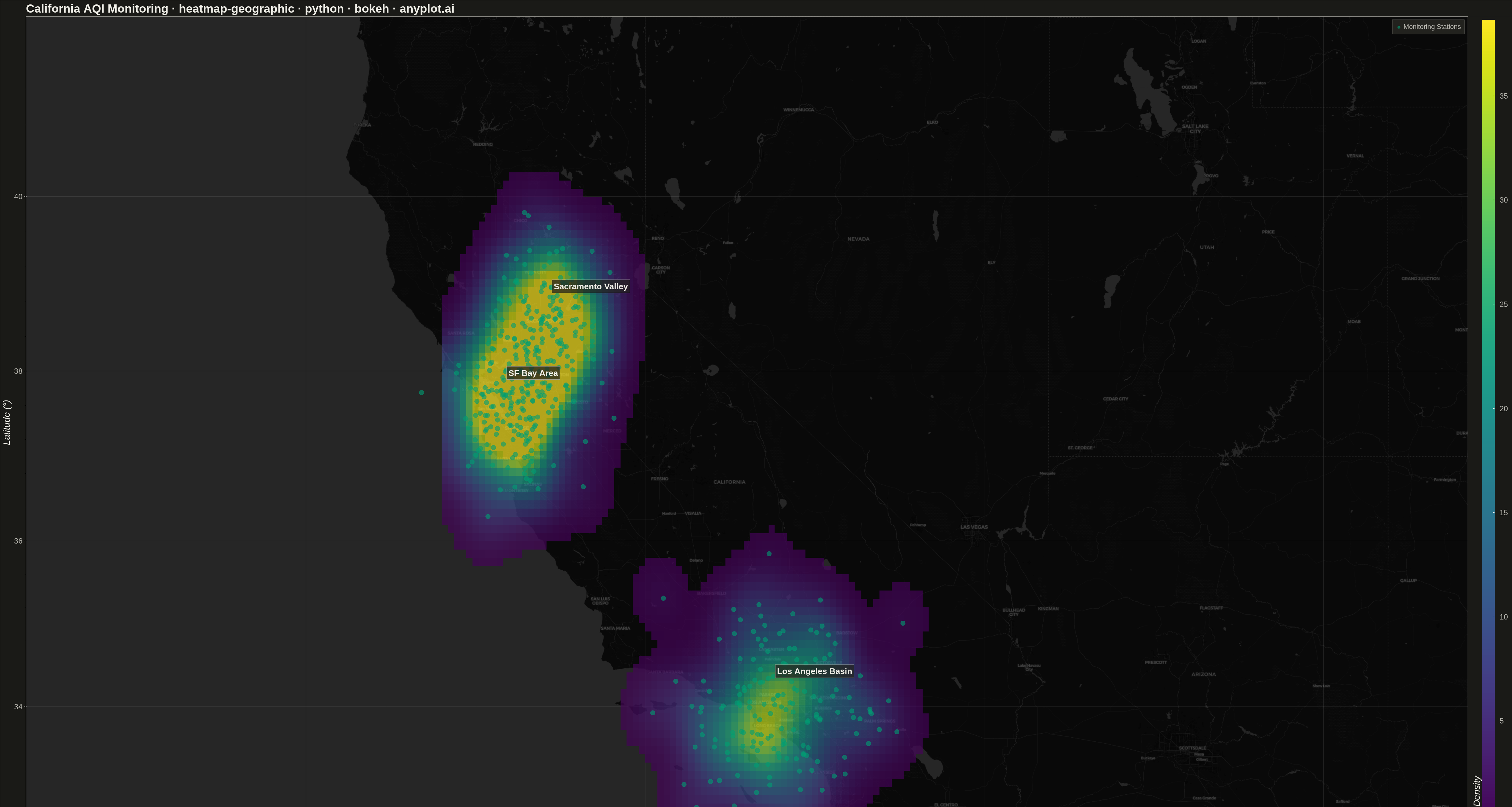
A geographic heatmap visualizes spatial density or intensity values across a map using continuous color gradients. Unlike choropleth maps that color discrete regions, this plot shows smooth density variations computed from point data or gridded values. The color intensity at each location represents the concentration or magnitude of the underlying data, making it ideal for identifying hotspots, clusters, and spatial patterns in geographic data.
""" anyplot.ai
heatmap-geographic: Geographic Heatmap for Spatial Density
Library: bokeh 3.9.0 | Python 3.13.13
Quality: 87/100 | Updated: 2026-05-18
"""

import sys
from pathlib import Path


script_dir = str(Path(__file__).parent.absolute())
sys.path = [p for p in sys.path if p != script_dir and p != ""]

import os
import time

import numpy as np
from bokeh.io import output_file, save
from bokeh.models import (
    BasicTicker,
    ColorBar,
    ColumnDataSource,
    HoverTool,
    LinearColorMapper,
    WMTSTileSource,
)
from bokeh.palettes import Viridis256
from bokeh.plotting import figure
from selenium import webdriver
from selenium.webdriver.chrome.options import Options


# Theme tokens
THEME = os.getenv("ANYPLOT_THEME", "light")
PAGE_BG = "#FAF8F1" if THEME == "light" else "#1A1A17"
ELEVATED_BG = "#FFFDF6" if THEME == "light" else "#242420"
INK = "#1A1A17" if THEME == "light" else "#F0EFE8"
INK_SOFT = "#4A4A44" if THEME == "light" else "#B8B7B0"
BRAND = "#009E73"  # Okabe-Ito position 1

# Data: Simulated environmental monitoring stations across California
np.random.seed(42)

n_points = 500

# Create clusters representing different monitoring regions
coast_lat = np.random.normal(36.5, 0.8, n_points // 3)
coast_lon = np.random.normal(-121.0, 0.5, n_points // 3)

socal_lat = np.random.normal(34.0, 0.6, n_points // 3)
socal_lon = np.random.normal(-118.0, 0.7, n_points // 3)

norcal_lat = np.random.normal(38.5, 0.5, n_points // 3 + n_points % 3)
norcal_lon = np.random.normal(-121.5, 0.4, n_points // 3 + n_points % 3)

latitudes = np.concatenate([coast_lat, socal_lat, norcal_lat])
longitudes = np.concatenate([coast_lon, socal_lon, norcal_lon])
values = np.random.exponential(scale=50, size=len(latitudes)) + 20

# Convert lat/lon to Web Mercator projection
merc_x = longitudes * 20037508.34 / 180
merc_y = np.log(np.tan((90 + latitudes) * np.pi / 360)) / (np.pi / 180) * 20037508.34 / 180

source = ColumnDataSource(data={"x": merc_x, "y": merc_y, "lat": latitudes, "lon": longitudes, "value": values})

# Map boundaries focused on California
lat_min, lat_max = 32.5, 42.0
lon_min, lon_max = -123.0, -114.0
x_min = lon_min * 20037508.34 / 180
x_max = lon_max * 20037508.34 / 180
y_min = np.log(np.tan((90 + lat_min) * np.pi / 360)) / (np.pi / 180) * 20037508.34 / 180
y_max = np.log(np.tan((90 + lat_max) * np.pi / 360)) / (np.pi / 180) * 20037508.34 / 180

# Create 2D histogram for density estimation
grid_resolution = 100
x_bins = np.linspace(x_min, x_max, grid_resolution)
y_bins = np.linspace(y_min, y_max, grid_resolution)

heatmap, x_edges, y_edges = np.histogram2d(merc_x, merc_y, bins=[x_bins, y_bins], weights=values, density=False)

# Apply Gaussian smoothing for continuous appearance
sigma = 3
kernel_size = int(6 * sigma + 1)
if kernel_size % 2 == 0:
    kernel_size += 1
kernel_x_arr = np.arange(kernel_size) - kernel_size // 2
kernel_1d = np.exp(-(kernel_x_arr**2) / (2 * sigma**2))
kernel_1d = kernel_1d / kernel_1d.sum()

heatmap_smooth = np.apply_along_axis(lambda row: np.convolve(row, kernel_1d, mode="same"), axis=0, arr=heatmap)
heatmap_smooth = np.apply_along_axis(lambda col: np.convolve(col, kernel_1d, mode="same"), axis=1, arr=heatmap_smooth)

# Plot
p = figure(
    width=4800,
    height=2700,
    x_range=(x_min, x_max),
    y_range=(y_min, y_max),
    x_axis_type="mercator",
    y_axis_type="mercator",
    title="California AQI Monitoring · heatmap-geographic · python · bokeh · anyplot.ai",
)

# Theme-appropriate basemap tile
if THEME == "light":
    tile_url = "https://cartodb-basemaps-a.global.ssl.fastly.net/light_all/{z}/{x}/{y}.png"
else:
    tile_url = "https://cartodb-basemaps-a.global.ssl.fastly.net/dark_all/{z}/{x}/{y}.png"
tile_source = WMTSTileSource(url=tile_url)
p.add_tile(tile_source)

# Heatmap color mapper using viridis for perceptually uniform density representation
max_density = np.percentile(heatmap_smooth[heatmap_smooth > 0], 95) if np.any(heatmap_smooth > 0) else 1
color_mapper = LinearColorMapper(palette=Viridis256, low=0, high=max_density, nan_color="rgba(0, 0, 0, 0)")

heatmap_display = heatmap_smooth.copy()
heatmap_display[heatmap_display < max_density * 0.01] = np.nan

p.image(
    image=[heatmap_display.T],
    x=x_min,
    y=y_min,
    dw=x_max - x_min,
    dh=y_max - y_min,
    color_mapper=color_mapper,
    alpha=0.7,
)

# Scatter monitoring stations with Okabe-Ito first series color
station_renderer = p.scatter(
    x="x", y="y", source=source, size=12, color=BRAND, alpha=0.6, legend_label="Monitoring Stations"
)

# HoverTool for interactive station details
hover = HoverTool(
    renderers=[station_renderer], tooltips=[("AQI Value", "@value{0.0}"), ("Lat / Lon", "@lat{0.00}° / @lon{0.00}°")]
)
p.add_tools(hover)

# Colorbar with larger title for visibility at canvas scale
color_bar = ColorBar(
    color_mapper=color_mapper,
    ticker=BasicTicker(),
    label_standoff=16,
    border_line_color=None,
    location=(0, 0),
    title="AQI Density",
    title_text_font_size="22pt",
    title_text_color=INK,
    major_label_text_font_size="18pt",
    major_label_text_color=INK_SOFT,
    width=40,
    background_fill_color=PAGE_BG,
)
p.add_layout(color_bar, "right")

# Theme-adaptive chrome
p.background_fill_color = PAGE_BG
p.border_fill_color = PAGE_BG
p.outline_line_color = INK_SOFT

p.title.text_font_size = "28pt"
p.title.text_color = INK

p.xaxis.axis_label = "Longitude (°)"
p.yaxis.axis_label = "Latitude (°)"
p.xaxis.axis_label_text_font_size = "22pt"
p.yaxis.axis_label_text_font_size = "22pt"
p.xaxis.axis_label_text_color = INK
p.yaxis.axis_label_text_color = INK
p.xaxis.major_label_text_font_size = "18pt"
p.yaxis.major_label_text_font_size = "18pt"
p.xaxis.major_label_text_color = INK_SOFT
p.yaxis.major_label_text_color = INK_SOFT
p.xaxis.axis_line_color = INK_SOFT
p.yaxis.axis_line_color = INK_SOFT
p.xaxis.major_tick_line_color = INK_SOFT
p.yaxis.major_tick_line_color = INK_SOFT

p.xgrid.grid_line_color = INK
p.ygrid.grid_line_color = INK
p.xgrid.grid_line_alpha = 0.10
p.ygrid.grid_line_alpha = 0.10

p.legend.location = "top_right"
p.legend.label_text_font_size = "16pt"
p.legend.background_fill_color = ELEVATED_BG
p.legend.border_line_color = INK_SOFT
p.legend.label_text_color = INK_SOFT

# Save HTML (required catalog artifact)
output_file(f"plot-{THEME}.html", title="Geographic Heatmap for Spatial Density")
save(p)

# Screenshot with headless Chrome via Selenium
W, H = 4800, 2700
opts = Options()
for arg in (
    "--headless=new",
    "--no-sandbox",
    "--disable-dev-shm-usage",
    "--disable-gpu",
    f"--window-size={W},{H}",
    "--hide-scrollbars",
):
    opts.add_argument(arg)
driver = webdriver.Chrome(options=opts)
driver.set_window_size(W, H)
driver.get(f"file://{Path(f'plot-{THEME}.html').resolve()}")
time.sleep(3)
driver.save_screenshot(f"plot-{THEME}.png")
driver.quit()
Runnable source as JSON, for any HTTP client: https://api.anyplot.ai/specs/heatmap-geographic/bokeh/code. Any spec id and library id listed in llms-full.txt fit the same URL shape; every URL below is complete and callable.
{
  "spec_id": "heatmap-geographic",
  "language": "python",
  "library": "bokeh",
  "page": "https://anyplot.ai/heatmap-geographic/python/bokeh",
  "hub": "https://anyplot.ai/heatmap-geographic",
  "code_json": "https://api.anyplot.ai/specs/heatmap-geographic/bokeh/code",
  "spec_json": "https://api.anyplot.ai/specs/heatmap-geographic",
  "render_light_png": "https://storage.googleapis.com/anyplot-images/plots/heatmap-geographic/python/bokeh/plot-light.png",
  "render_dark_png": "https://storage.googleapis.com/anyplot-images/plots/heatmap-geographic/python/bokeh/plot-dark.png",
  "interactive_light_html": "https://storage.googleapis.com/anyplot-images/plots/heatmap-geographic/python/bokeh/plot-light.html",
  "interactive_dark_html": "https://storage.googleapis.com/anyplot-images/plots/heatmap-geographic/python/bokeh/plot-dark.html",
  "quality_score": 87.0,
  "license": "MIT",
  "guide": "https://anyplot.ai/llms.txt"
}
Part of Geographic Heatmap for Spatial Density on anyplot.ai.