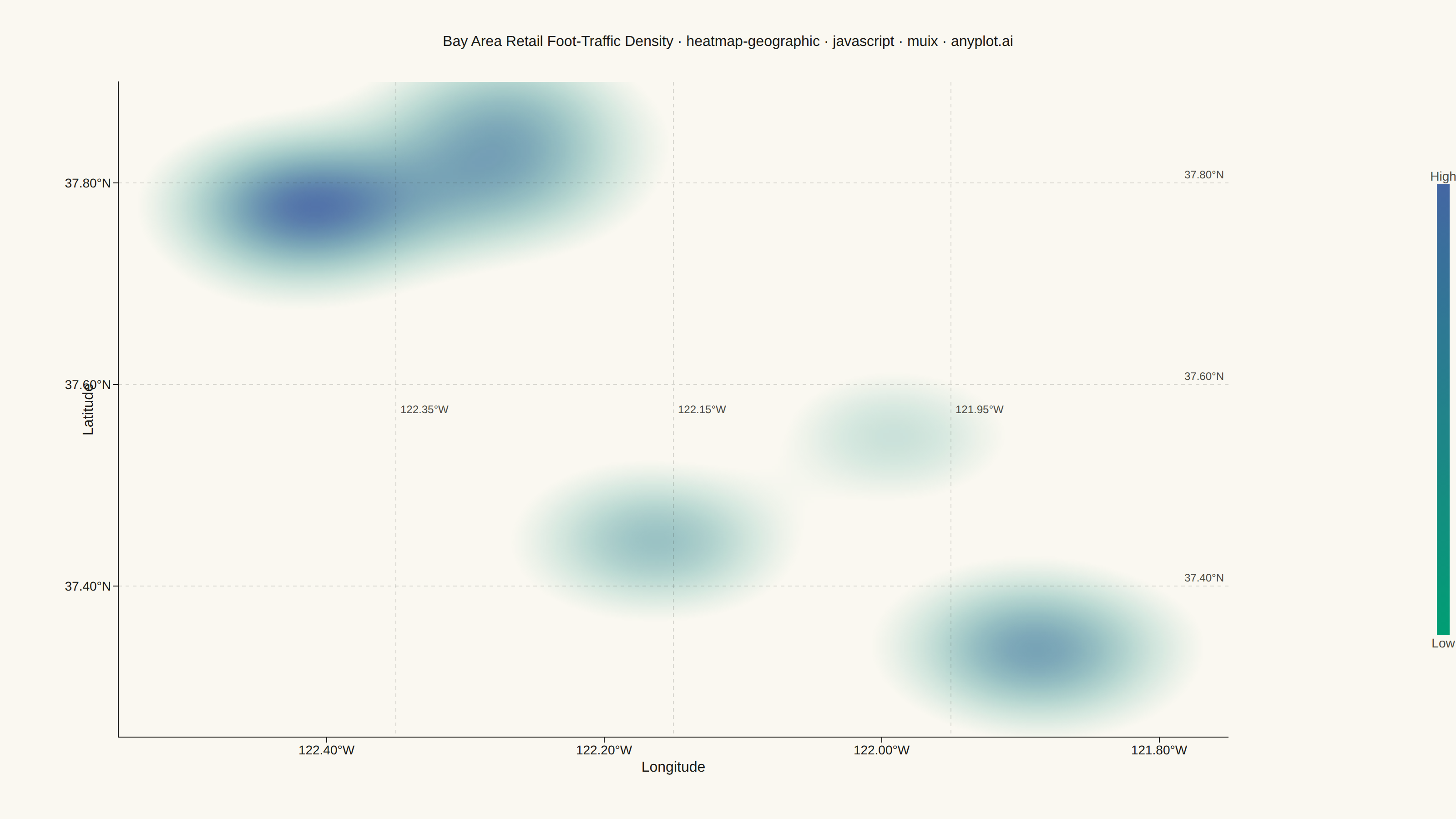
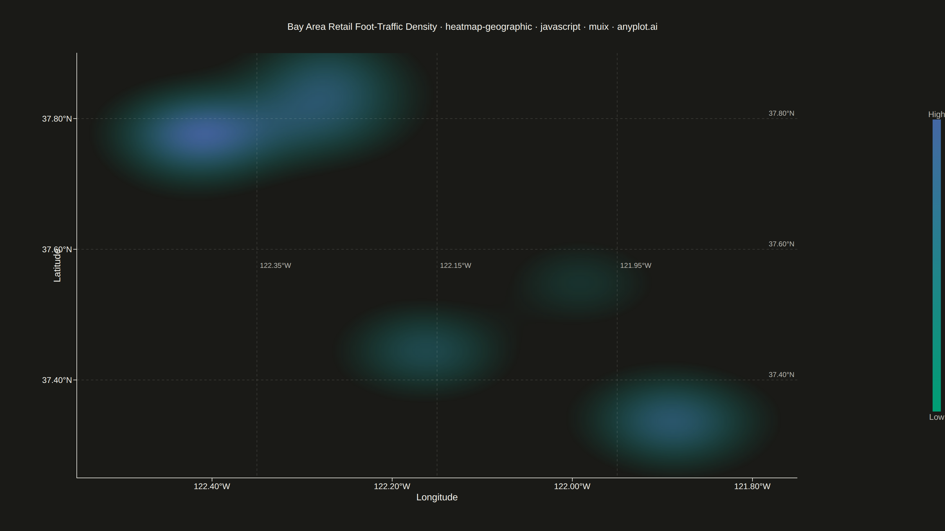
The same plot in 14 other libraries — JavaScript: Chart.js, D3.js, Apache ECharts, Highcharts; Python: Altair, Bokeh, lets-plot, Matplotlib, Plotly, plotnine, Pygal, Seaborn; R: ggplot2; Julia: Makie.jl. Compare all 15 side by side: Geographic Heatmap for Spatial Density in Python, R, Julia and JavaScript.
A geographic heatmap visualizes spatial density or intensity values across a map using continuous color gradients. Unlike choropleth maps that color discrete regions, this plot shows smooth density variations computed from point data or gridded values. The color intensity at each location represents the concentration or magnitude of the underlying data, making it ideal for identifying hotspots, clusters, and spatial patterns in geographic data.
// anyplot.ai
// heatmap-geographic: Geographic Heatmap for Spatial Density
// Library: muix 7.29.1 | JavaScript 22.23.2
// Quality: 88/100 | Created: 2026-09-02
import { ScatterChart } from "@mui/x-charts/ScatterChart";
import { ContinuousColorLegend } from "@mui/x-charts/ChartsLegend";
import { ChartsReferenceLine } from "@mui/x-charts/ChartsReferenceLine";

const t = window.ANYPLOT_TOKENS;
const SIZE = window.ANYPLOT_SIZE;
const MARGIN = { top: 90, right: 250, bottom: 90, left: 130 };
const PLOT_WIDTH = SIZE.width - MARGIN.left - MARGIN.right;
const PLOT_HEIGHT = SIZE.height - MARGIN.top - MARGIN.bottom;

const TITLE =
  "Bay Area Retail Foot-Traffic Density · heatmap-geographic · javascript · muix · anyplot.ai";
// Scale the title down once it runs past the ~67-char mandated baseline
// (see prompts/plot-generator.md "Title fontsize must scale with title length").
const TITLE_FONT_SIZE = Math.max(14, Math.round(22 * Math.min(1, 67 / TITLE.length)));

// --- Deterministic PRNG (fixed-seed LCG, Box-Muller for gaussian jitter) ----
let seed = 42;
const rand = () => {
  seed = (seed * 1664525 + 1013904223) % 4294967296;
  return seed / 4294967296;
};
const gaussian = () => {
  const u1 = Math.max(rand(), 1e-9);
  const u2 = rand();
  return Math.sqrt(-2 * Math.log(u1)) * Math.cos(2 * Math.PI * u2);
};

// --- Data: retail foot-traffic check-ins across the San Francisco Bay Area --
const LON_MIN = -122.55;
const LON_MAX = -121.75;
const LAT_MIN = 37.25;
const LAT_MAX = 37.9;

// Degrees-to-km conversion at this latitude, used so the KDE bandwidth below
// reflects real city-scale distances instead of raw (anisotropic) degrees.
const KM_PER_DEG_LAT = 111;
const KM_PER_DEG_LON = 88;

const hotspots = [
  { lon: -122.42, lat: 37.775, weight: 1.0, sigmaKm: 2.6 }, // San Francisco downtown
  { lon: -122.27, lat: 37.805, weight: 0.7, sigmaKm: 3.2 }, // Oakland downtown
  { lon: -122.27, lat: 37.872, weight: 0.4, sigmaKm: 2.2 }, // Berkeley
  { lon: -121.885, lat: 37.335, weight: 0.85, sigmaKm: 3.4 }, // San Jose downtown
  { lon: -122.16, lat: 37.445, weight: 0.55, sigmaKm: 2.4 }, // Palo Alto
  { lon: -121.99, lat: 37.548, weight: 0.3, sigmaKm: 2.0 }, // Fremont
];

const visits = [];
hotspots.forEach((h) => {
  const count = Math.round(h.weight * 140);
  for (let i = 0; i < count; i += 1) {
    visits.push({
      lon: h.lon + (gaussian() * h.sigmaKm) / KM_PER_DEG_LON,
      lat: h.lat + (gaussian() * h.sigmaKm) / KM_PER_DEG_LAT,
    });
  }
});
for (let i = 0; i < 90; i += 1) {
  visits.push({
    lon: LON_MIN + rand() * (LON_MAX - LON_MIN),
    lat: LAT_MIN + rand() * (LAT_MAX - LAT_MIN),
  });
}

// --- Kernel density estimate, rasterized to a smooth image ------------------
// A discrete-marker scatter approximation leaves scalloped circular edges
// around each hotspot. Community @mui/x-charts has no native heatmap/image
// layer, so instead the KDE is sampled onto a raster grid, colour-mapped per
// pixel (Imprint sequential ramp, alpha fading out below DENSITY_FLOOR), and
// drawn as one <image>: the browser's own bilinear upscaling then renders a
// genuinely continuous density field. Distances are converted to km so the
// kernel is isotropic in real space, and truncated at 3*bandwidth so
// far-away points can't sum into a visible tail.
const BANDWIDTH_KM = 4.5;
const TRUNC_KM_SQ = (3 * BANDWIDTH_KM) ** 2;
const DENSITY_FLOOR = 0.12; // below this the pixel is fully transparent
const RASTER_W = 400;
const RASTER_H = Math.round(RASTER_W * (PLOT_HEIGHT / PLOT_WIDTH));

const rawDensity = new Float32Array(RASTER_W * RASTER_H);
let maxDensity = 0;
for (let py = 0; py < RASTER_H; py += 1) {
  const lat = LAT_MAX - ((py + 0.5) / RASTER_H) * (LAT_MAX - LAT_MIN);
  for (let px = 0; px < RASTER_W; px += 1) {
    const lon = LON_MIN + ((px + 0.5) / RASTER_W) * (LON_MAX - LON_MIN);
    let density = 0;
    for (let i = 0; i < visits.length; i += 1) {
      const dKmLon = (lon - visits[i].lon) * KM_PER_DEG_LON;
      const dKmLat = (lat - visits[i].lat) * KM_PER_DEG_LAT;
      const distKmSq = dKmLon * dKmLon + dKmLat * dKmLat;
      if (distKmSq < TRUNC_KM_SQ) {
        density += Math.exp(-distKmSq / (2 * BANDWIDTH_KM * BANDWIDTH_KM));
      }
    }
    rawDensity[py * RASTER_W + px] = density;
    maxDensity = Math.max(maxDensity, density);
  }
}

const hexToRgb = (hex) => [
  parseInt(hex.slice(1, 3), 16),
  parseInt(hex.slice(3, 5), 16),
  parseInt(hex.slice(5, 7), 16),
];
const seqLowRgb = hexToRgb(t.seq[0]);
const seqHighRgb = hexToRgb(t.seq[1]);

const canvas = document.createElement("canvas");
canvas.width = RASTER_W;
canvas.height = RASTER_H;
const ctx = canvas.getContext("2d");
const image = ctx.createImageData(RASTER_W, RASTER_H);
for (let i = 0; i < rawDensity.length; i += 1) {
  const z = Math.min(1, rawDensity[i] / maxDensity);
  const o = i * 4;
  image.data[o] = Math.round(seqLowRgb[0] + (seqHighRgb[0] - seqLowRgb[0]) * z);
  image.data[o + 1] = Math.round(seqLowRgb[1] + (seqHighRgb[1] - seqLowRgb[1]) * z);
  image.data[o + 2] = Math.round(seqLowRgb[2] + (seqHighRgb[2] - seqLowRgb[2]) * z);
  image.data[o + 3] =
    z <= DENSITY_FLOOR ? 0 : Math.round(((z - DENSITY_FLOOR) / (1 - DENSITY_FLOOR)) * 235);
}
ctx.putImageData(image, 0, 0);
const HEATMAP_URI = canvas.toDataURL("image/png");

// --- Geographic reference graticule (basemap substitute — no map tiles are
// available in the community package, so a lon/lat grid gives spatial context)
const latLines = [37.4, 37.6, 37.8];
const lonLines = [-122.35, -122.15, -121.95];

function MapTitle() {
  return (
    <text
      x={SIZE.width / 2}
      y={40}
      textAnchor="middle"
      dominantBaseline="hanging"
      fontSize={TITLE_FONT_SIZE}
      fontWeight={500}
      fill={t.ink}
    >
      {TITLE}
    </text>
  );
}

export default function Chart() {
  return (
    <ScatterChart
      width={SIZE.width}
      height={SIZE.height}
      skipAnimation
      disableVoronoi
      margin={MARGIN}
      series={[]}
      xAxis={[
        {
          min: LON_MIN,
          max: LON_MAX,
          label: "Longitude",
          tickNumber: 4,
          valueFormatter: (v) => `${Math.abs(v).toFixed(2)}°W`,
          tickLabelStyle: { fontSize: 14 },
          labelStyle: { fontSize: 16 },
        },
      ]}
      yAxis={[
        {
          min: LAT_MIN,
          max: LAT_MAX,
          label: "Latitude",
          tickNumber: 4,
          valueFormatter: (v) => `${v.toFixed(2)}°N`,
          tickLabelStyle: { fontSize: 14 },
          labelStyle: { fontSize: 16 },
        },
      ]}
      zAxis={[
        {
          id: "density",
          min: 0,
          max: 1,
          // min/max must also live on colorMap itself: ContinuousColorLegend
          // reads colorMap.min/max directly (not the axis-level min/max).
          colorMap: { type: "continuous", min: 0, max: 1, color: [t.seq[0], t.seq[1]] },
        },
      ]}
      slots={{ noDataOverlay: () => null }}
      slotProps={{ legend: { hidden: true } }}
    >
      <image
        href={HEATMAP_URI}
        x={MARGIN.left}
        y={MARGIN.top}
        width={PLOT_WIDTH}
        height={PLOT_HEIGHT}
        preserveAspectRatio="none"
      />
      {latLines.map((lat) => (
        <ChartsReferenceLine
          key={`lat-${lat}`}
          y={lat}
          lineStyle={{ stroke: t.grid, strokeDasharray: "4 4", strokeWidth: 1 }}
          label={`${lat.toFixed(2)}°N`}
          labelStyle={{ fontSize: 12, fill: t.inkSoft }}
          labelAlign="end"
        />
      ))}
      {lonLines.map((lon) => (
        <ChartsReferenceLine
          key={`lon-${lon}`}
          x={lon}
          lineStyle={{ stroke: t.grid, strokeDasharray: "4 4", strokeWidth: 1 }}
          label={`${Math.abs(lon).toFixed(2)}°W`}
          labelStyle={{ fontSize: 12, fill: t.inkSoft }}
        />
      ))}
      <ContinuousColorLegend
        axisDirection="z"
        axisId="density"
        position={{ horizontal: "right", vertical: "middle" }}
        direction="column"
        length="55%"
        thickness={14}
        minLabel="Low"
        maxLabel="High"
        labelStyle={{ fontSize: 14, fill: t.inkSoft }}
      />
      <MapTitle />
    </ScatterChart>
  );
}
Runnable source as JSON, for any HTTP client: https://api.anyplot.ai/specs/heatmap-geographic/muix/code. Any spec id and library id listed in llms-full.txt fit the same URL shape; every URL below is complete and callable.
{
  "spec_id": "heatmap-geographic",
  "language": "javascript",
  "library": "muix",
  "page": "https://anyplot.ai/heatmap-geographic/javascript/muix",
  "hub": "https://anyplot.ai/heatmap-geographic",
  "code_json": "https://api.anyplot.ai/specs/heatmap-geographic/muix/code",
  "spec_json": "https://api.anyplot.ai/specs/heatmap-geographic",
  "render_light_png": "https://storage.googleapis.com/anyplot-images/plots/heatmap-geographic/javascript/muix/plot-light.png",
  "render_dark_png": "https://storage.googleapis.com/anyplot-images/plots/heatmap-geographic/javascript/muix/plot-dark.png",
  "interactive_light_html": "https://storage.googleapis.com/anyplot-images/plots/heatmap-geographic/javascript/muix/plot-light.html",
  "interactive_dark_html": "https://storage.googleapis.com/anyplot-images/plots/heatmap-geographic/javascript/muix/plot-dark.html",
  "quality_score": 88.0,
  "license": "MIT",
  "guide": "https://anyplot.ai/llms.txt"
}
Part of Geographic Heatmap for Spatial Density on anyplot.ai.