The same plot in 14 other libraries — Python: Altair, Bokeh, lets-plot, Matplotlib, Plotly, plotnine, Pygal, Seaborn; R: ggplot2; JavaScript: Chart.js, D3.js, Apache ECharts, Highcharts, MUI X Charts. Compare all 15 side by side: Geographic Heatmap for Spatial Density in Python, R, Julia and JavaScript.
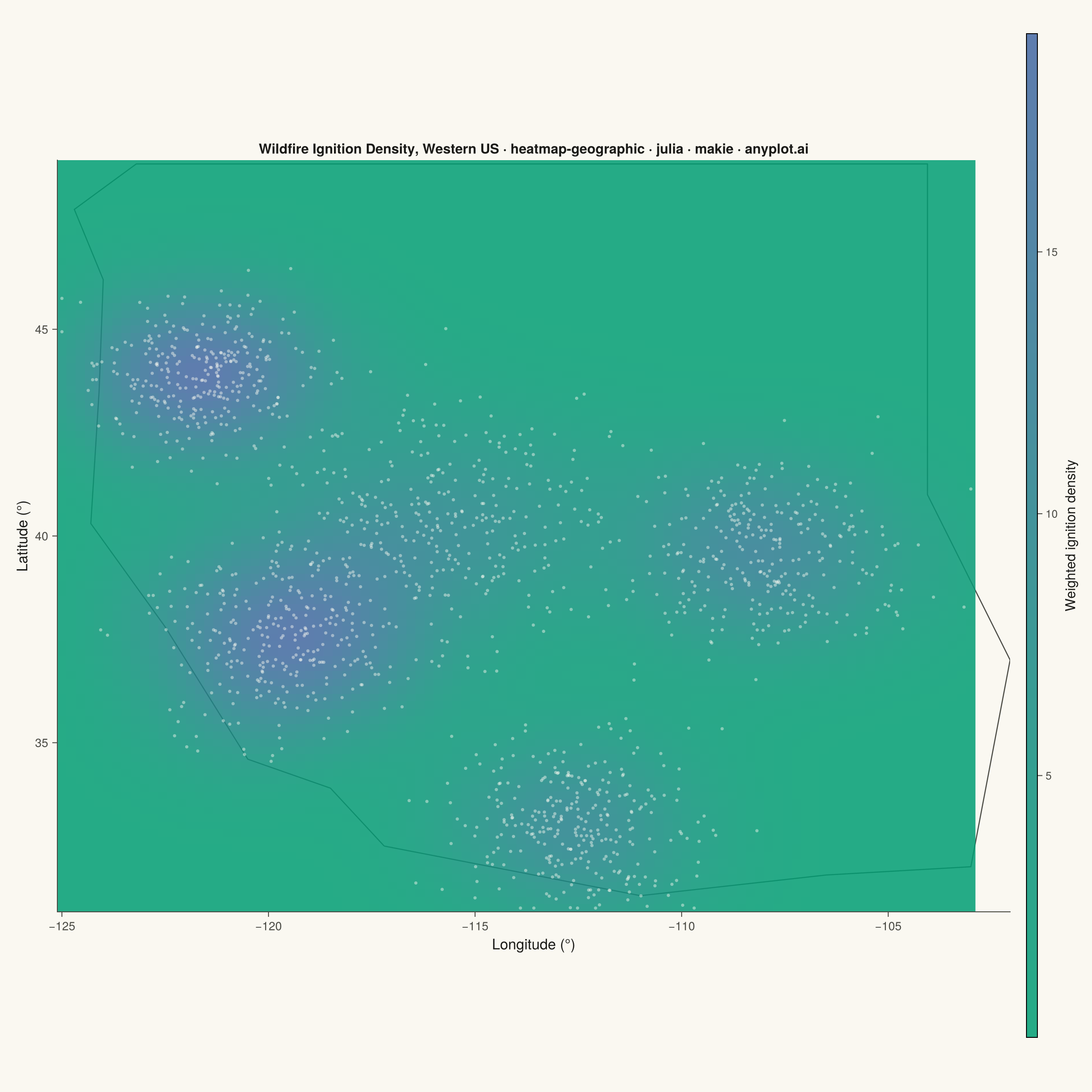
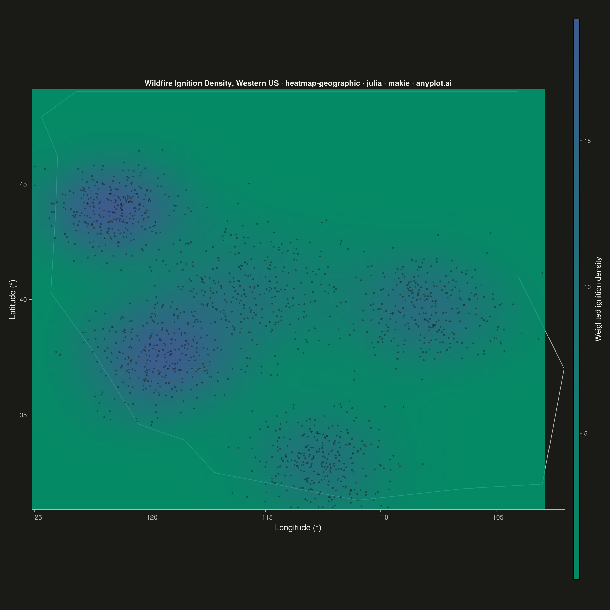
A geographic heatmap visualizes spatial density or intensity values across a map using continuous color gradients. Unlike choropleth maps that color discrete regions, this plot shows smooth density variations computed from point data or gridded values. The color intensity at each location represents the concentration or magnitude of the underlying data, making it ideal for identifying hotspots, clusters, and spatial patterns in geographic data.
# anyplot.ai
# heatmap-geographic: Geographic Heatmap for Spatial Density
# Library: makie 0.21.9 | Julia 1.11.9
# Quality: 87/100 | Created: 2026-09-02

using CairoMakie
using Colors
using Random
using Statistics

Random.seed!(42)

# --- Theme tokens -----------------------------------------------------------
THEME    = get(ENV, "ANYPLOT_THEME", "light")
PAGE_BG  = THEME == "light" ? colorant"#FAF8F1" : colorant"#1A1A17"
INK      = THEME == "light" ? colorant"#1A1A17" : colorant"#F0EFE8"
INK_SOFT = THEME == "light" ? colorant"#4A4A44" : colorant"#B8B7B0"

# Imprint sequential colormap — density is single-polarity (never negative)
ANYPLOT_SEQ = cgrad([colorant"#009E73", colorant"#4467A3"])

# --- Data: simulated wildfire ignitions across the western US ---------------
# Bounding box for the plotted region
LON_MIN, LON_MAX = -125.0, -103.0
LAT_MIN, LAT_MAX = 31.0, 49.0

# Wildfire-prone regions with an average burn severity (acres) per cluster
cluster_lon      = [-119.5, -121.5, -108.0, -116.0, -112.5]
cluster_lat      = [37.5, 44.0, 39.5, 40.5, 33.0]
cluster_spread   = [1.6, 1.3, 1.7, 1.9, 1.4]
cluster_severity = [320.0, 260.0, 220.0, 190.0, 160.0]
points_per_cluster = 300

longitudes = Float64[]
latitudes = Float64[]
acres_burned = Float64[]
for c in 1:length(cluster_lon)
    append!(longitudes, cluster_lon[c] .+ cluster_spread[c] .* randn(points_per_cluster))
    append!(latitudes, cluster_lat[c] .+ 0.75 * cluster_spread[c] .* randn(points_per_cluster))
    append!(acres_burned, cluster_severity[c] .* exp.(0.6 .* randn(points_per_cluster)))
end
longitudes = clamp.(longitudes, LON_MIN, LON_MAX)
latitudes = clamp.(latitudes, LAT_MIN, LAT_MAX)
n_points = length(longitudes)
weights = acres_burned ./ mean(acres_burned)

# --- Simplified western-US geographic context (Pacific coastline + national
# borders) — a small set of hardcoded boundary points, no GeoMakie needed ----
boundary_lon = [-117.2, -118.5, -120.5, -122.5, -124.3, -124.1, -124.0, -124.7,
    -123.2, -116.0, -104.05, -104.05, -104.05, -102.05, -103.0, -106.5, -111.0, -117.2]
boundary_lat = [32.5, 33.9, 34.6, 37.8, 40.3, 43.5, 46.2, 47.9,
    49.0, 49.0, 49.0, 45.0, 41.0, 37.0, 32.0, 31.8, 31.3, 32.5]

# --- Kernel density estimation on a regular lon/lat grid ---------------------
# Silverman's rule of thumb bandwidth, per dimension
bw_lon = std(longitudes) * n_points^(-1 / 6)
bw_lat = std(latitudes) * n_points^(-1 / 6)

grid_n = 100
lon_grid = range(LON_MIN, LON_MAX; length=grid_n)
lat_grid = range(LAT_MIN, LAT_MAX; length=grid_n)
norm_factor = 1.0 / (2 * pi * bw_lon * bw_lat)

# Broadcast the (grid_n,) squared-distance vectors into a (grid_n, grid_n)
# outer-sum matrix per point, accumulating over points — avoids a manual
# triple-nested loop while keeping the same grid_n × grid_n × n_points cost.
density = zeros(grid_n, grid_n)
for k in 1:n_points
    dx2 = ((lon_grid .- longitudes[k]) ./ bw_lon) .^ 2
    dy2 = ((lat_grid .- latitudes[k]) ./ bw_lat) .^ 2
    density .+= weights[k] .* exp.(-0.5 .* (dx2 .+ dy2'))
end
density .*= norm_factor

# --- Title (fontsize scales down once the descriptive prefix pushes past the
# ~67-char mandated-title baseline) -------------------------------------------
title_str = "Wildfire Ignition Density, Western US · heatmap-geographic · julia · makie · anyplot.ai"
title_ratio = length(title_str) > 67 ? 67 / length(title_str) : 1.0
title_size = round(Int, 20 * title_ratio)

# --- Plot ---------------------------------------------------------------------
fig = Figure(
    resolution      = (1200, 1200),
    fontsize        = 14,
    backgroundcolor = PAGE_BG,
)

ax = Axis(
    fig[1, 1];
    title             = title_str,
    titlesize         = title_size,
    titlecolor        = INK,
    xlabel            = "Longitude (°)",
    ylabel            = "Latitude (°)",
    xlabelsize        = 16,
    ylabelsize        = 16,
    xlabelcolor       = INK,
    ylabelcolor       = INK,
    xticklabelsize    = 13,
    yticklabelsize    = 13,
    xticklabelcolor   = INK_SOFT,
    yticklabelcolor   = INK_SOFT,
    xtickcolor        = INK_SOFT,
    ytickcolor        = INK_SOFT,
    backgroundcolor   = PAGE_BG,
    aspect            = DataAspect(),
    topspinevisible   = false,
    rightspinevisible = false,
    leftspinecolor    = INK_SOFT,
    bottomspinecolor  = INK_SOFT,
    xgridvisible      = false,
    ygridvisible      = false,
)

# Basemap: simplified coastline/border outline, drawn first so the
# semi-transparent density layer shows it through underneath
lines!(ax, boundary_lon, boundary_lat; color=INK_SOFT, linewidth=1.2)

hm = heatmap!(ax, lon_grid, lat_grid, density; colormap=ANYPLOT_SEQ, alpha=0.85)

# Raw ignition points, faint, for spatial context under the density layer
scatter!(ax, longitudes, latitudes;
    color       = (PAGE_BG, 0.45),
    markersize  = 5,
    strokewidth = 0,
)

Colorbar(fig[1, 2], hm;
    label          = "Weighted ignition density",
    labelsize      = 15,
    labelcolor     = INK,
    ticklabelsize  = 12,
    ticklabelcolor = INK_SOFT,
    tickcolor      = INK_SOFT,
)

# --- Save ---------------------------------------------------------------------
save("plot-$(THEME).png", fig; px_per_unit=2)
Runnable source as JSON, for any HTTP client: https://api.anyplot.ai/specs/heatmap-geographic/makie/code. Any spec id and library id listed in llms-full.txt fit the same URL shape; every URL below is complete and callable.
{
  "spec_id": "heatmap-geographic",
  "language": "julia",
  "library": "makie",
  "page": "https://anyplot.ai/heatmap-geographic/julia/makie",
  "hub": "https://anyplot.ai/heatmap-geographic",
  "code_json": "https://api.anyplot.ai/specs/heatmap-geographic/makie/code",
  "spec_json": "https://api.anyplot.ai/specs/heatmap-geographic",
  "render_light_png": "https://storage.googleapis.com/anyplot-images/plots/heatmap-geographic/julia/makie/plot-light.png",
  "render_dark_png": "https://storage.googleapis.com/anyplot-images/plots/heatmap-geographic/julia/makie/plot-dark.png",
  "quality_score": 87.0,
  "license": "MIT",
  "guide": "https://anyplot.ai/llms.txt"
}
Part of Geographic Heatmap for Spatial Density on anyplot.ai.