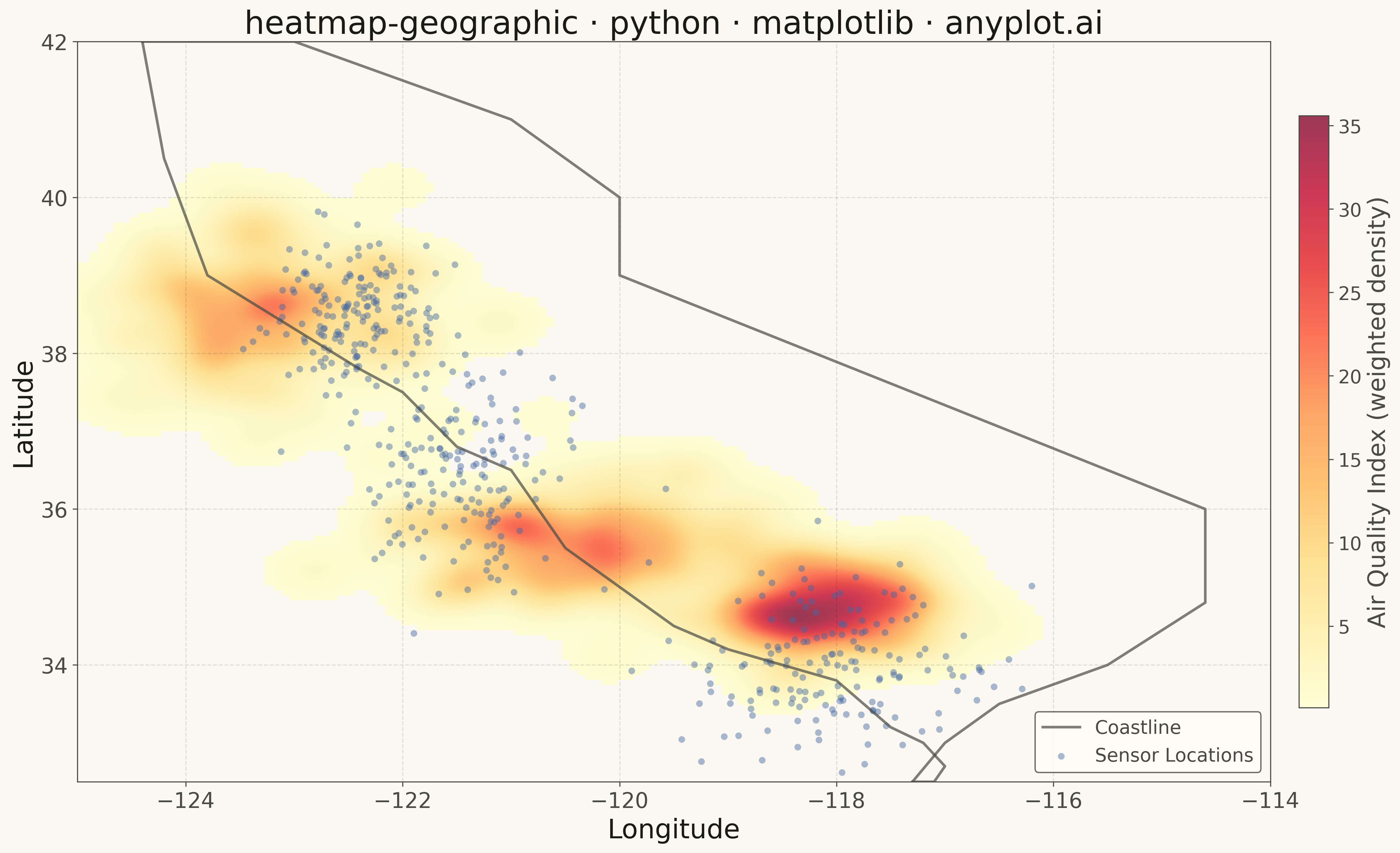
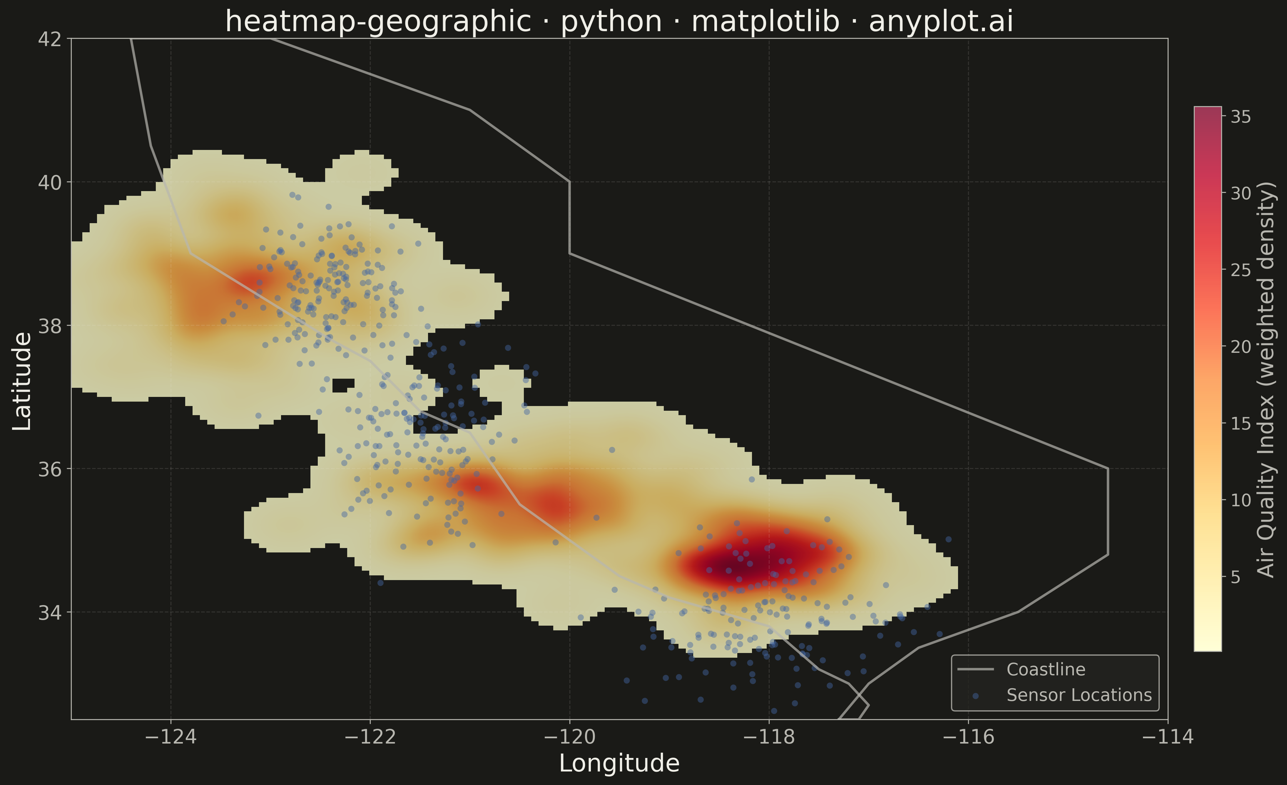
A geographic heatmap visualizes spatial density or intensity values across a map using continuous color gradients. Unlike choropleth maps that color discrete regions, this plot shows smooth density variations computed from point data or gridded values. The color intensity at each location represents the concentration or magnitude of the underlying data, making it ideal for identifying hotspots, clusters, and spatial patterns in geographic data.
""" anyplot.ai
heatmap-geographic: Geographic Heatmap for Spatial Density
Library: matplotlib 3.10.9 | Python 3.13.13
Quality: 82/100 | Updated: 2026-05-19
"""

import os

import matplotlib.pyplot as plt
import numpy as np


# Theme tokens
THEME = os.getenv("ANYPLOT_THEME", "light")
PAGE_BG = "#FAF8F1" if THEME == "light" else "#1A1A17"
ELEVATED_BG = "#FFFDF6" if THEME == "light" else "#242420"
INK = "#1A1A17" if THEME == "light" else "#F0EFE8"
INK_SOFT = "#4A4A44" if THEME == "light" else "#B8B7B0"
INK_MUTED = "#6B6A63" if THEME == "light" else "#A8A79F"

# Data: Simulated environmental monitoring stations across California
np.random.seed(42)

n_points = 500

# Create clusters representing different monitoring regions
coast_lat = np.random.normal(36.5, 0.8, n_points // 3)
coast_lon = np.random.normal(-121.5, 0.5, n_points // 3)

socal_lat = np.random.normal(34.0, 0.6, n_points // 3)
socal_lon = np.random.normal(-118.0, 0.7, n_points // 3)

norcal_lat = np.random.normal(38.5, 0.5, n_points // 3 + n_points % 3)
norcal_lon = np.random.normal(-122.5, 0.4, n_points // 3 + n_points % 3)

latitudes = np.concatenate([coast_lat, socal_lat, norcal_lat])
longitudes = np.concatenate([coast_lon, socal_lon, norcal_lon])

# AQI values: realistic range 0–150 (Good to Unhealthy)
values = np.clip(np.random.gamma(shape=2.5, scale=28, size=len(latitudes)), 5, 150)

# Define map boundaries for California
lat_min, lat_max = 32.5, 42.0
lon_min, lon_max = -125.0, -114.0

# Create 2D histogram for density estimation
grid_resolution = 150
lat_bins = np.linspace(lat_min, lat_max, grid_resolution)
lon_bins = np.linspace(lon_min, lon_max, grid_resolution)

heatmap, lat_edges, lon_edges = np.histogram2d(
    latitudes, longitudes, bins=[lat_bins, lon_bins], weights=values, density=False
)

# Gaussian smoothing for continuous appearance (KDE approximation)
sigma = 3
kernel_size = int(6 * sigma + 1)
if kernel_size % 2 == 0:
    kernel_size += 1
kernel_x = np.arange(kernel_size) - kernel_size // 2
kernel_1d = np.exp(-(kernel_x**2) / (2 * sigma**2))
kernel_1d = kernel_1d / kernel_1d.sum()

heatmap_smooth = np.apply_along_axis(lambda row: np.convolve(row, kernel_1d, mode="same"), axis=0, arr=heatmap)
heatmap_smooth = np.apply_along_axis(lambda col: np.convolve(col, kernel_1d, mode="same"), axis=1, arr=heatmap_smooth)

# Mask zero/near-zero values for transparency
heatmap_masked = np.ma.masked_where(heatmap_smooth < 0.1, heatmap_smooth)

# Plot
fig, ax = plt.subplots(figsize=(16, 9), facecolor=PAGE_BG)
ax.set_facecolor(PAGE_BG)

# California outline approximation
coast_lons = [
    -124.4,
    -124.2,
    -123.8,
    -122.4,
    -122.0,
    -121.5,
    -121.0,
    -120.5,
    -120.0,
    -119.5,
    -119.0,
    -118.5,
    -118.0,
    -117.5,
    -117.2,
    -117.0,
    -117.1,
    -117.3,
]
coast_lats = [
    42.0,
    40.5,
    39.0,
    37.8,
    37.5,
    36.8,
    36.5,
    35.5,
    35.0,
    34.5,
    34.2,
    34.0,
    33.8,
    33.2,
    33.0,
    32.7,
    32.5,
    32.5,
]
ax.plot(coast_lons, coast_lats, color=INK_SOFT, linewidth=2, alpha=0.7, label="Coastline")

east_lons = [-117.3, -117.0, -116.5, -115.5, -114.6, -114.6, -120.0, -120.0, -121.0, -122.0, -123.0, -124.2, -124.4]
east_lats = [32.5, 33.0, 33.5, 34.0, 34.8, 36.0, 39.0, 40.0, 41.0, 41.5, 42.0, 42.0, 42.0]
ax.plot(east_lons, east_lats, color=INK_SOFT, linewidth=2, alpha=0.7)

# Heatmap layer
extent = [lon_min, lon_max, lat_min, lat_max]
im = ax.imshow(
    heatmap_masked.T, extent=extent, origin="lower", aspect="auto", cmap="YlOrRd", alpha=0.78, interpolation="bilinear"
)

# Sensor locations (slightly more visible than before)
ax.scatter(longitudes, latitudes, s=25, c="#4467A3", alpha=0.45, edgecolors="none", label="Sensor Locations")

# Colorbar
cbar = plt.colorbar(im, ax=ax, shrink=0.8, pad=0.02)
cbar.set_label("Air Quality Index (weighted density)", fontsize=18, color=INK_SOFT)
cbar.ax.tick_params(labelsize=14, colors=INK_SOFT)
cbar.outline.set_edgecolor(INK_SOFT)

# Style
ax.set_xlabel("Longitude", fontsize=20, color=INK)
ax.set_ylabel("Latitude", fontsize=20, color=INK)
ax.set_title("heatmap-geographic · python · matplotlib · anyplot.ai", fontsize=24, fontweight="medium", color=INK)
ax.tick_params(axis="both", labelsize=16, colors=INK_SOFT)
ax.set_xlim(lon_min, lon_max)
ax.set_ylim(lat_min, lat_max)

for spine in ax.spines.values():
    spine.set_color(INK_SOFT)

ax.grid(True, alpha=0.12, linestyle="--", color=INK)

# Legend positioned in lower right to avoid overlap with dense northern clusters
leg = ax.legend(loc="lower right", fontsize=14)
leg.get_frame().set_facecolor(ELEVATED_BG)
leg.get_frame().set_edgecolor(INK_SOFT)
plt.setp(leg.get_texts(), color=INK_SOFT)

plt.tight_layout()
plt.savefig(f"plot-{THEME}.png", dpi=300, bbox_inches="tight", facecolor=PAGE_BG)
Runnable source as JSON, for any HTTP client: https://api.anyplot.ai/specs/heatmap-geographic/matplotlib/code. Any spec id and library id listed in llms-full.txt fit the same URL shape; every URL below is complete and callable.
{
  "spec_id": "heatmap-geographic",
  "language": "python",
  "library": "matplotlib",
  "page": "https://anyplot.ai/heatmap-geographic/python/matplotlib",
  "hub": "https://anyplot.ai/heatmap-geographic",
  "code_json": "https://api.anyplot.ai/specs/heatmap-geographic/matplotlib/code",
  "spec_json": "https://api.anyplot.ai/specs/heatmap-geographic",
  "render_light_png": "https://storage.googleapis.com/anyplot-images/plots/heatmap-geographic/python/matplotlib/plot-light.png",
  "render_dark_png": "https://storage.googleapis.com/anyplot-images/plots/heatmap-geographic/python/matplotlib/plot-dark.png",
  "quality_score": 82.0,
  "license": "MIT",
  "guide": "https://anyplot.ai/llms.txt"
}
Part of Geographic Heatmap for Spatial Density on anyplot.ai.