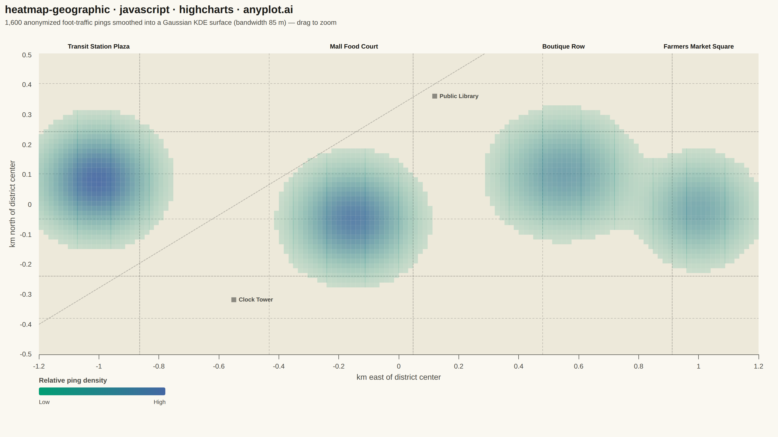
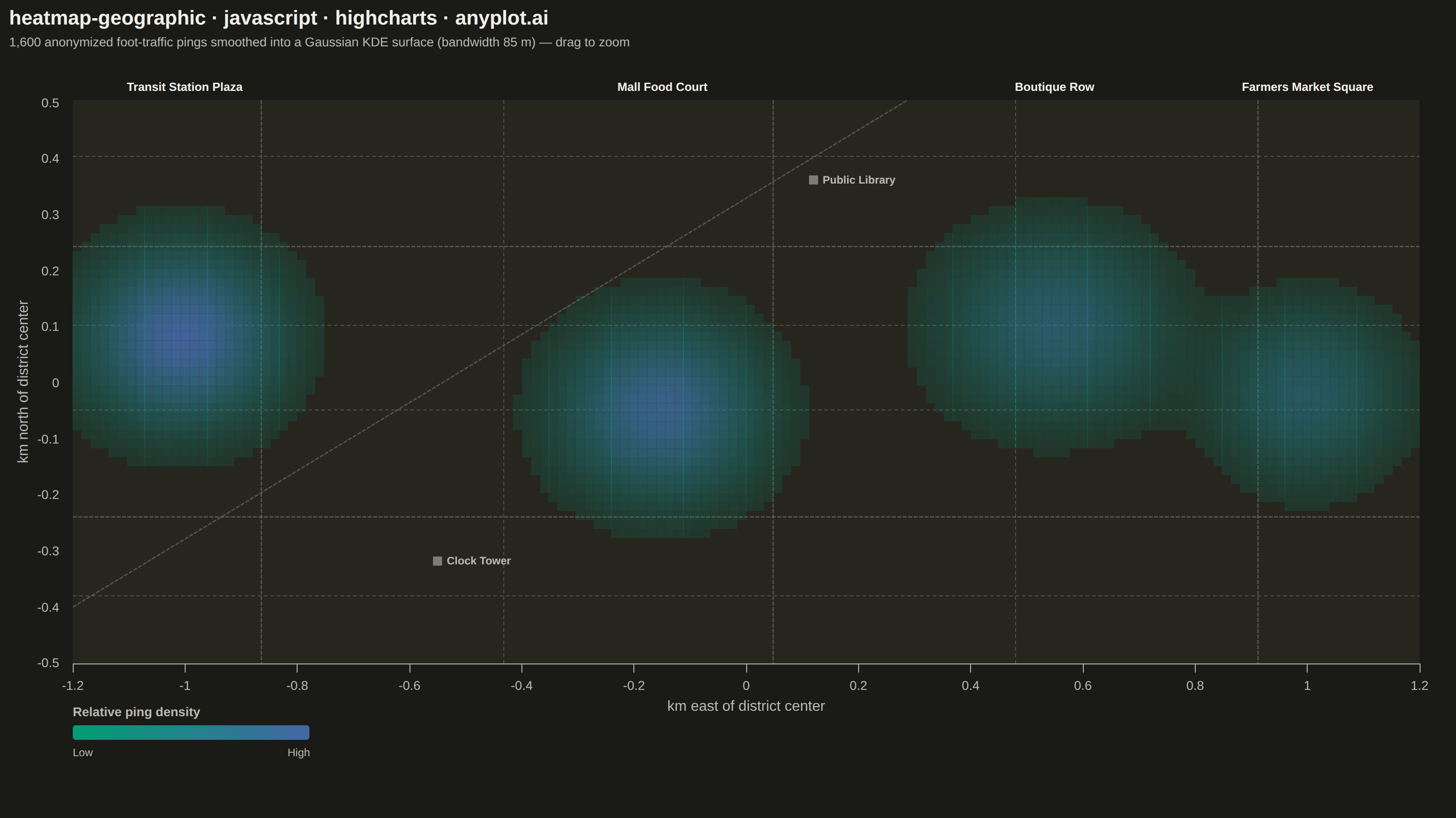
The same plot in 14 other libraries — JavaScript: Chart.js, D3.js, Apache ECharts, MUI X Charts; Python: Altair, Bokeh, lets-plot, Matplotlib, Plotly, plotnine, Pygal, Seaborn; R: ggplot2; Julia: Makie.jl. Compare all 15 side by side: Geographic Heatmap for Spatial Density in Python, R, Julia and JavaScript.
A geographic heatmap visualizes spatial density or intensity values across a map using continuous color gradients. Unlike choropleth maps that color discrete regions, this plot shows smooth density variations computed from point data or gridded values. The color intensity at each location represents the concentration or magnitude of the underlying data, making it ideal for identifying hotspots, clusters, and spatial patterns in geographic data.
// anyplot.ai
// heatmap-geographic: Geographic Heatmap for Spatial Density
// Library: highcharts 12.6.0 | JavaScript 22.23.2
// Quality: 92/100 | Created: 2026-09-02

const t = window.ANYPLOT_TOKENS;
const THEME = window.ANYPLOT_THEME;

// --- Basemap chrome (not data — Imprint palette only governs data colors) --
const BLOCK_FILL = THEME === "light" ? "#EDE9DA" : "#26261F";
const STREET_COLOR = THEME === "light" ? "rgba(107,106,99,0.4)" : "rgba(168,167,159,0.35)";

// --- Layout constants --------------------------------------------------------
// The mount is a fixed 1600×900 CSS box (harness renders at deviceScaleFactor 2
// -> 3200×1800 PNG). Margins are set explicitly so the plot-area pixel size is
// known at codegen time, letting a district bounding box be chosen whose aspect
// ratio matches plotWidth/plotHeight — that keeps the density grid cells square
// instead of stretched (1 km must map to the same pixel count on both axes).
const MOUNT_WIDTH = 1600;
const MOUNT_HEIGHT = 900;
const MARGIN_LEFT = 80;
const MARGIN_RIGHT = 40;
const MARGIN_TOP = 110;
const MARGIN_BOTTOM = 170; // x-axis title/ticks + gap + hand-drawn gradient legend
const PLOT_WIDTH = MOUNT_WIDTH - MARGIN_LEFT - MARGIN_RIGHT;
const PLOT_HEIGHT = MOUNT_HEIGHT - MARGIN_TOP - MARGIN_BOTTOM;

// Illustrative shopping-street district, not a real place.
const LAT0 = 45.42;
const LON0 = -75.7;
const KM_PER_DEG_LAT = 110.57;
const KM_PER_DEG_LON = 111.32 * Math.cos((LAT0 * Math.PI) / 180);

const X_RANGE_KM = 2.4; // district width — a long commercial corridor
const Y_RANGE_KM = (X_RANGE_KM * PLOT_HEIGHT) / PLOT_WIDTH; // locks pixel aspect
const X_MIN = -X_RANGE_KM / 2;
const X_MAX = X_RANGE_KM / 2;
const Y_MIN = -Y_RANGE_KM / 2;
const Y_MAX = Y_RANGE_KM / 2;
const PX_PER_KM = PLOT_WIDTH / X_RANGE_KM;

// --- Deterministic PRNG (browser has no seeded RNG) --------------------------
let lcgState = 42;
function nextRandom() {
  lcgState = (lcgState * 1103515245 + 12345) % 2147483648;
  return lcgState / 2147483648;
}
function jitter(spread) {
  // Sum of 3 uniforms centred on 0 — cheap approx-normal, bounded, deterministic.
  return ((nextRandom() + nextRandom() + nextRandom() - 1.5) / 1.5) * spread;
}

// --- Data: anonymized, opted-in foot-traffic pings near a shopping district --
// (latitude, longitude) only — value defaults to 1, i.e. pure point density,
// as used for retail site-selection analysis.
const HOTSPOTS = [
  { name: "Transit Station Plaza", cx: -1.0, cy: 0.08, spread: 0.14, weight: 0.34 },
  { name: "Mall Food Court", cx: -0.15, cy: -0.05, spread: 0.16, weight: 0.3 },
  { name: "Boutique Row", cx: 0.55, cy: 0.1, spread: 0.22, weight: 0.22 },
  { name: "Farmers Market Square", cx: 1.0, cy: -0.02, spread: 0.12, weight: 0.14 },
];
const N_PINGS = 1600;

// Fixed landmark reference points (away from every hotspot) so the basemap
// reads as a real district layout, not just a density surface.
const LANDMARKS = [
  { name: "Clock Tower", x: -0.55, y: -0.32 },
  { name: "Public Library", x: 0.12, y: 0.36 },
];

const pings = [];
HOTSPOTS.forEach((hotspot) => {
  const target = Math.round(N_PINGS * hotspot.weight);
  for (let i = 0; i < target; i++) {
    const x = hotspot.cx + jitter(hotspot.spread);
    const y = hotspot.cy + jitter(hotspot.spread * 0.6);
    if (x < X_MIN || x > X_MAX || y < Y_MIN || y > Y_MAX) continue;
    pings.push({
      x,
      y,
      lat: Math.round((LAT0 + y / KM_PER_DEG_LAT) * 10000) / 10000,
      lon: Math.round((LON0 + x / KM_PER_DEG_LON) * 10000) / 10000,
    });
  }
});

// --- Kernel density estimation on a regular grid -----------------------------
// A Gaussian KDE turns the discrete pings into the continuous intensity surface
// the spec calls for (as opposed to e.g. hexagonal binning). BANDWIDTH_KM sets
// how far each ping's influence spreads — tuned to this district's ~2.4 km
// scale so adjacent hotspots blend smoothly without merging into one blob.
const BANDWIDTH_KM = 0.085;
const GRID_COLS = 150;
const CELL_KM = X_RANGE_KM / GRID_COLS;
const GRID_ROWS = Math.round(Y_RANGE_KM / CELL_KM);
const CELL_PX = PX_PER_KM * CELL_KM;
const TWO_BW_SQ = 2 * BANDWIDTH_KM * BANDWIDTH_KM;
const CUTOFF_KM = 3.2 * BANDWIDTH_KM; // skip pings beyond ~3.2 sigma — negligible contribution

let maxDensity = 0;
const cells = [];
for (let row = 0; row < GRID_ROWS; row++) {
  const cy = Y_MIN + (row + 0.5) * CELL_KM;
  for (let col = 0; col < GRID_COLS; col++) {
    const cx = X_MIN + (col + 0.5) * CELL_KM;
    let density = 0;
    for (let p = 0; p < pings.length; p++) {
      const dx = pings[p].x - cx;
      if (dx > CUTOFF_KM || dx < -CUTOFF_KM) continue;
      const dy = pings[p].y - cy;
      if (dy > CUTOFF_KM || dy < -CUTOFF_KM) continue;
      density += Math.exp(-(dx * dx + dy * dy) / TWO_BW_SQ);
    }
    if (density > maxDensity) maxDensity = density;
    cells.push({ x: cx, y: cy, density });
  }
}

// --- Map density -> Imprint sequential gradient + alpha ----------------------
// The core Highcharts bundle has no heatmap/colorAxis module (see
// prompts/library/highcharts.md), so each cell's fill is computed by hand — a
// gamma-boosted interpolation across the two-stop imprint_seq gradient, with
// alpha scaling so near-zero cells stay transparent and the basemap shows
// through underneath (per spec: "sequential colormap ... with transparency").
const seqLow = [t.seq[0].slice(1, 3), t.seq[0].slice(3, 5), t.seq[0].slice(5, 7)].map((h) => parseInt(h, 16));
const seqHigh = [t.seq[1].slice(1, 3), t.seq[1].slice(3, 5), t.seq[1].slice(5, 7)].map((h) => parseInt(h, 16));
const MIN_ALPHA = 0.04;
const MAX_ALPHA = 0.92;
const RENDER_THRESHOLD = 0.03; // skip visually-negligible cells (basemap already shows through)

const heatCells = [];
cells.forEach((cell) => {
  const frac = maxDensity > 0 ? cell.density / maxDensity : 0;
  if (frac < RENDER_THRESHOLD) return;
  const boosted = Math.pow(frac, 0.6); // lifts mid-range density into visible contrast
  const rgb = seqLow.map((c, i) => Math.round(c + (seqHigh[i] - c) * boosted));
  const alpha = MIN_ALPHA + (MAX_ALPHA - MIN_ALPHA) * boosted;
  heatCells.push({
    x: cell.x,
    y: cell.y,
    lat: Math.round((LAT0 + cell.y / KM_PER_DEG_LAT) * 10000) / 10000,
    lon: Math.round((LON0 + cell.x / KM_PER_DEG_LON) * 10000) / 10000,
    frac: Math.round(frac * 1000) / 1000,
    color: `rgba(${rgb[0]},${rgb[1]},${rgb[2]},${alpha.toFixed(3)})`,
  });
});

// --- Schematic street grid — basemap context beneath the density surface ----
// Irregular spacing plus major/minor line weights (avenues vs. side streets)
// and one diagonal boulevard, so the basemap reads as an actual district
// layout rather than a uniform grid. Each line is its own tiny series (not one
// multi-segment series) so Highcharts never re-sorts the two endpoints by x,
// which would otherwise scramble the grid.
const STREET_LINE_BASE = {
  type: "line",
  color: STREET_COLOR,
  marker: { enabled: false },
  enableMouseTracking: false,
  showInLegend: false,
  zIndex: 0,
};
const AVENUE_STYLE = { lineWidth: 1.5, dashStyle: "ShortDash" }; // major streets
const SIDE_STREET_STYLE = { lineWidth: 1, dashStyle: "Dash" }; // minor streets
const AVENUE_X_FRACS = [0.14, 0.52, 0.88];
const SIDE_STREET_X_FRACS = [0.32, 0.7];
const AVENUE_Y_FRACS = [0.26, 0.74];
const SIDE_STREET_Y_FRACS = [0.12, 0.45, 0.6, 0.9];
const streetGridSeries = [
  ...AVENUE_X_FRACS.map((f) => ({
    ...STREET_LINE_BASE,
    ...AVENUE_STYLE,
    data: [
      [X_MIN + f * X_RANGE_KM, Y_MAX],
      [X_MIN + f * X_RANGE_KM, Y_MIN],
    ],
  })),
  ...SIDE_STREET_X_FRACS.map((f) => ({
    ...STREET_LINE_BASE,
    ...SIDE_STREET_STYLE,
    data: [
      [X_MIN + f * X_RANGE_KM, Y_MAX],
      [X_MIN + f * X_RANGE_KM, Y_MIN],
    ],
  })),
  ...AVENUE_Y_FRACS.map((f) => ({
    ...STREET_LINE_BASE,
    ...AVENUE_STYLE,
    data: [
      [X_MIN, Y_MIN + f * Y_RANGE_KM],
      [X_MAX, Y_MIN + f * Y_RANGE_KM],
    ],
  })),
  ...SIDE_STREET_Y_FRACS.map((f) => ({
    ...STREET_LINE_BASE,
    ...SIDE_STREET_STYLE,
    data: [
      [X_MIN, Y_MIN + f * Y_RANGE_KM],
      [X_MAX, Y_MIN + f * Y_RANGE_KM],
    ],
  })),
  {
    ...STREET_LINE_BASE,
    ...AVENUE_STYLE,
    data: [
      [X_MIN, Y_MIN + 0.1 * Y_RANGE_KM],
      [X_MIN + 0.62 * X_RANGE_KM, Y_MAX],
    ],
  }, // diagonal boulevard cutting across the grid
];

// --- Chart --------------------------------------------------------------------
const title = "heatmap-geographic · javascript · highcharts · anyplot.ai";

function drawColorLegend(chart) {
  const r = chart.renderer;
  const x0 = chart.plotLeft;
  const y0 = chart.plotTop + chart.plotHeight + 68;
  const barWidth = 260;
  const barHeight = 16;

  r.text("Relative ping density", x0, y0 - 10)
    .css({ color: t.inkSoft, fontSize: "14px", fontWeight: "600" })
    .add();

  r.rect(x0, y0, barWidth, barHeight, 3)
    .attr({
      fill: {
        linearGradient: { x1: 0, y1: 0, x2: 1, y2: 0 },
        stops: [
          [0, t.seq[0]],
          [1, t.seq[1]],
        ],
      },
      "stroke-width": 0,
    })
    .add();
  r.text("Low", x0, y0 + barHeight + 18)
    .css({ color: t.inkSoft, fontSize: "12px" })
    .add();
  r.text("High", x0 + barWidth - 24, y0 + barHeight + 18)
    .css({ color: t.inkSoft, fontSize: "12px" })
    .add();
}

// Named on the chart directly, turning the color contrast into a story instead
// of leaving it to the tooltip alone. Placed in the margin band above the plot
// area since the density surface can extend right up to the axis-max edge.
function drawHotspotLabels(chart) {
  const py = chart.plotTop - 10;
  HOTSPOTS.forEach((h) => {
    const px = chart.xAxis[0].toPixels(h.cx, false);
    chart.renderer
      .text(h.name, px, py)
      .attr({ align: "center" })
      .css({ color: t.ink, fontSize: "13px", fontWeight: "700" })
      .add();
  });
}

// Two fixed landmark markers (small filled square + label) reinforce that the
// basemap represents a real street layout, distinct from the density blobs.
function drawLandmarks(chart) {
  LANDMARKS.forEach((lm) => {
    const px = chart.xAxis[0].toPixels(lm.x, false);
    const py = chart.yAxis[0].toPixels(lm.y, false);
    chart.renderer.rect(px - 5, py - 5, 10, 10).attr({ fill: t.inkSoft, opacity: 0.6, "stroke-width": 0, zIndex: 2 }).add();
    chart.renderer
      .text(lm.name, px + 10, py + 4)
      .css({ color: t.inkSoft, fontSize: "12px", fontWeight: "600" })
      .add();
  });
}

Highcharts.chart(
  "container",
  {
    chart: {
      type: "scatter",
      backgroundColor: "transparent",
      plotBackgroundColor: BLOCK_FILL,
      animation: false,
      style: { fontFamily: "inherit" },
      marginLeft: MARGIN_LEFT,
      marginRight: MARGIN_RIGHT,
      marginTop: MARGIN_TOP,
      marginBottom: MARGIN_BOTTOM,
      zooming: { type: "xy" }, // interactive HTML: drag to zoom into any part of the surface
    },
    credits: { enabled: false },
    colors: t.palette,
    title: {
      text: title,
      align: "left",
      style: { color: t.ink, fontSize: "22px", fontWeight: "600" },
    },
    subtitle: {
      text: `${N_PINGS.toLocaleString()} anonymized foot-traffic pings smoothed into a Gaussian KDE surface (bandwidth ${Math.round(BANDWIDTH_KM * 1000)} m) — drag to zoom`,
      align: "left",
      style: { color: t.inkSoft, fontSize: "14px" },
    },
    xAxis: {
      min: X_MIN,
      max: X_MAX,
      startOnTick: false,
      endOnTick: false,
      title: { text: "km east of district center", style: { color: t.inkSoft, fontSize: "16px" } },
      lineColor: t.inkSoft,
      tickColor: t.inkSoft,
      gridLineWidth: 0,
      labels: { style: { color: t.inkSoft, fontSize: "14px" } },
    },
    yAxis: {
      min: Y_MIN,
      max: Y_MAX,
      startOnTick: false,
      endOnTick: false,
      title: { text: "km north of district center", style: { color: t.inkSoft, fontSize: "16px" } },
      lineColor: t.inkSoft,
      tickColor: t.inkSoft,
      gridLineWidth: 0,
      labels: { style: { color: t.inkSoft, fontSize: "14px" } },
    },
    legend: { enabled: false },
    tooltip: {
      backgroundColor: t.elevatedBg,
      borderColor: t.inkSoft,
      style: { color: t.ink, fontSize: "13px" },
      useHTML: false,
    },
    plotOptions: {
      series: { animation: false },
    },
    series: [
      ...streetGridSeries,
      {
        name: "Ping density",
        type: "scatter",
        data: heatCells,
        showInLegend: false,
        zIndex: 1,
        marker: {
          symbol: "square",
          radius: CELL_PX / 2,
          lineWidth: 0,
          states: { hover: { enabled: false } },
        },
        turboThreshold: 0,
        tooltip: {
          pointFormatter() {
            return (
              `Relative density: ${(this.frac * 100).toFixed(0)}%<br/>` +
              `≈ ${this.lat}°N, ${Math.abs(this.lon)}°W`
            );
          },
        },
      },
    ],
  },
  function (chart) {
    drawColorLegend(chart);
    drawHotspotLabels(chart);
    drawLandmarks(chart);
  },
);
Runnable source as JSON, for any HTTP client: https://api.anyplot.ai/specs/heatmap-geographic/highcharts/code. Any spec id and library id listed in llms-full.txt fit the same URL shape; every URL below is complete and callable.
{
  "spec_id": "heatmap-geographic",
  "language": "javascript",
  "library": "highcharts",
  "page": "https://anyplot.ai/heatmap-geographic/javascript/highcharts",
  "hub": "https://anyplot.ai/heatmap-geographic",
  "code_json": "https://api.anyplot.ai/specs/heatmap-geographic/highcharts/code",
  "spec_json": "https://api.anyplot.ai/specs/heatmap-geographic",
  "render_light_png": "https://storage.googleapis.com/anyplot-images/plots/heatmap-geographic/javascript/highcharts/plot-light.png",
  "render_dark_png": "https://storage.googleapis.com/anyplot-images/plots/heatmap-geographic/javascript/highcharts/plot-dark.png",
  "interactive_light_html": "https://storage.googleapis.com/anyplot-images/plots/heatmap-geographic/javascript/highcharts/plot-light.html",
  "interactive_dark_html": "https://storage.googleapis.com/anyplot-images/plots/heatmap-geographic/javascript/highcharts/plot-dark.html",
  "quality_score": 92.0,
  "license": "MIT",
  "guide": "https://anyplot.ai/llms.txt"
}
Part of Geographic Heatmap for Spatial Density on anyplot.ai.