The same plot in 14 other libraries — JavaScript: Chart.js, Apache ECharts, Highcharts, MUI X Charts; Python: Altair, Bokeh, lets-plot, Matplotlib, Plotly, plotnine, Pygal, Seaborn; R: ggplot2; Julia: Makie.jl. Compare all 15 side by side: 2D Histogram Heatmap in Python, R, Julia and JavaScript.
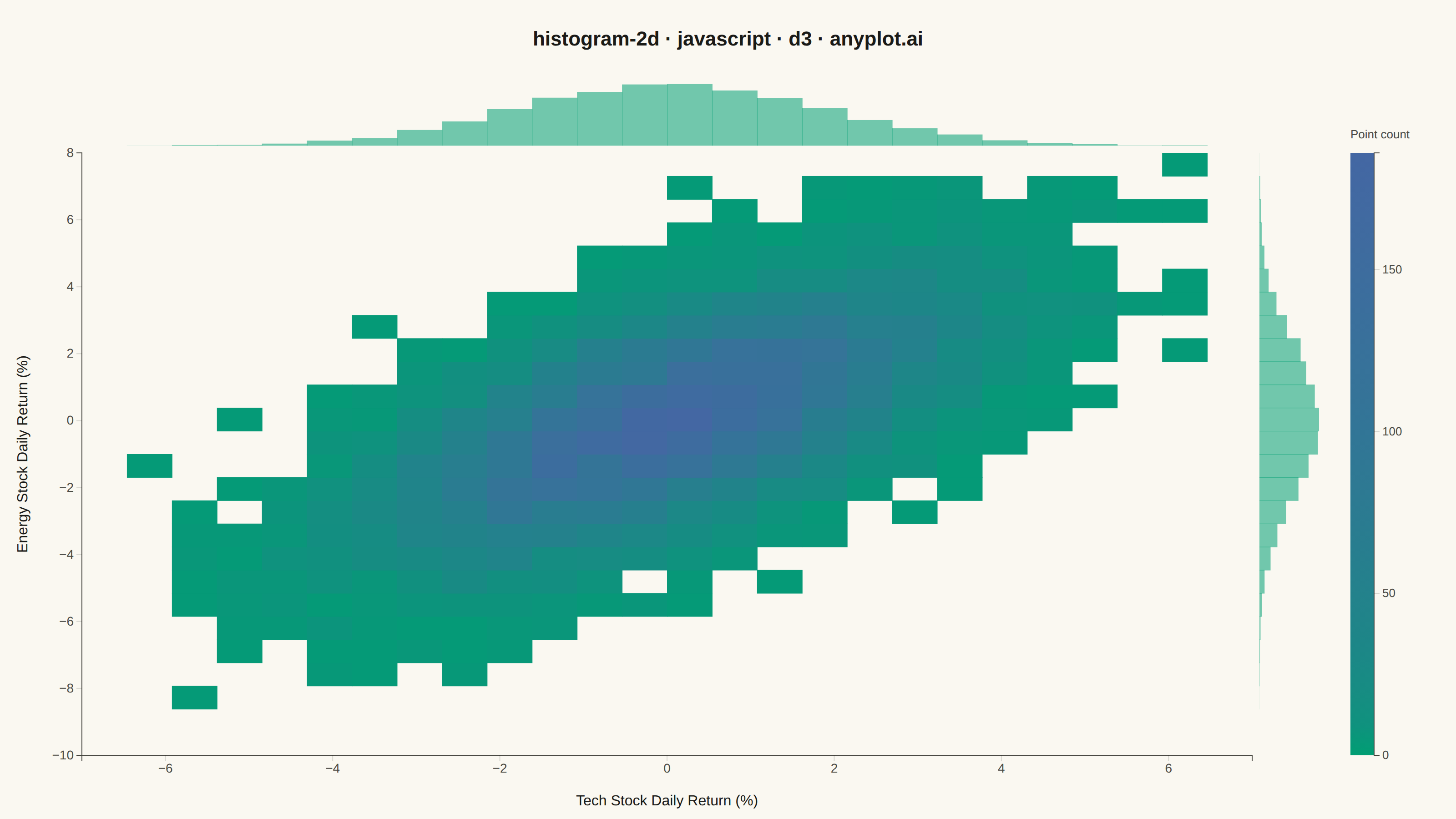
A two-dimensional histogram that displays the joint distribution of two continuous variables as a heatmap with rectangular bins. Each bin's color intensity represents the frequency or count of data points falling within that region, making it ideal for revealing density patterns, clusters, and correlations in bivariate data. Unlike scatter plots that can become cluttered with large datasets, 2D histograms effectively summarize point density.
// anyplot.ai
// histogram-2d: 2D Histogram Heatmap
// Library: d3 7.9.0 | JavaScript 22.23.2
// Quality: 86/100 | Created: 2026-09-05

const t = window.ANYPLOT_TOKENS;
const { width, height } = window.ANYPLOT_SIZE;

// --- Data (in-memory, deterministic bivariate normal via Box-Muller) -------
function mulberry32(seed) {
  return function () {
    seed |= 0;
    seed = (seed + 0x6d2b79f5) | 0;
    let z = Math.imul(seed ^ (seed >>> 15), 1 | seed);
    z = (z + Math.imul(z ^ (z >>> 7), 61 | z)) ^ z;
    return ((z ^ (z >>> 14)) >>> 0) / 4294967296;
  };
}

const rand = mulberry32(42);
const N_POINTS = 9000;
const CORRELATION = 0.65;
const MEAN_TECH = 0.05;
const STD_TECH = 1.8;
const MEAN_ENERGY = 0.03;
const STD_ENERGY = 2.2;

const points = [];
for (let i = 0; i < N_POINTS; i++) {
  const u1 = Math.max(rand(), 1e-12);
  const u2 = rand();
  const mag = Math.sqrt(-2 * Math.log(u1));
  const z0 = mag * Math.cos(2 * Math.PI * u2);
  const z1 = mag * Math.sin(2 * Math.PI * u2);
  const techReturn = MEAN_TECH + STD_TECH * z0;
  const energyReturn = MEAN_ENERGY + STD_ENERGY * (CORRELATION * z0 + Math.sqrt(1 - CORRELATION * CORRELATION) * z1);
  points.push({ x: techReturn, y: energyReturn });
}

// --- Binning (manual 2D grid — d3-array's bin() only handles 1D) -----------
const N_BINS = 26;
const [xMin, xMax] = d3.scaleLinear().domain(d3.extent(points, (d) => d.x)).nice().domain();
const [yMin, yMax] = d3.scaleLinear().domain(d3.extent(points, (d) => d.y)).nice().domain();
const xStep = (xMax - xMin) / N_BINS;
const yStep = (yMax - yMin) / N_BINS;

const counts = Array.from({ length: N_BINS }, () => new Array(N_BINS).fill(0));
for (const d of points) {
  const bx = Math.min(N_BINS - 1, Math.floor((d.x - xMin) / xStep));
  const by = Math.min(N_BINS - 1, Math.floor((d.y - yMin) / yStep));
  counts[bx][by] += 1;
}

const cells = [];
let maxCount = 0;
for (let bx = 0; bx < N_BINS; bx++) {
  for (let by = 0; by < N_BINS; by++) {
    const count = counts[bx][by];
    if (count > maxCount) maxCount = count;
    if (count > 0) cells.push({ bx, by, count });
  }
}

const xMarginal = counts.map((col) => d3.sum(col));
const yMarginal = d3.range(N_BINS).map((by) => d3.sum(counts.map((col) => col[by])));

// --- Layout (heatmap + top/right marginal histograms + colorbar) -----------
const gap = 8;
const mainX0 = 90;
const mainX1 = 1376;
const mainY0 = 168;
const mainY1 = 830;
const topMarginY0 = 90;
const topMarginY1 = mainY0 - gap;
const rightMarginX0 = mainX1 + gap;
const rightMarginX1 = rightMarginX0 + 70;
const colorbarX0 = rightMarginX1 + 30;
const colorbarX1 = colorbarX0 + 26;
const binWidthPx = (mainX1 - mainX0) / N_BINS;
const binHeightPx = (mainY1 - mainY0) / N_BINS;

const xScale = d3.scaleLinear().domain([xMin, xMax]).range([mainX0, mainX1]);
const yScale = d3.scaleLinear().domain([yMin, yMax]).range([mainY1, mainY0]);
const xMarginalScale = d3.scaleLinear().domain([0, d3.max(xMarginal)]).nice().range([topMarginY1, topMarginY0]);
const yMarginalScale = d3.scaleLinear().domain([0, d3.max(yMarginal)]).nice().range([rightMarginX0, rightMarginX1]);

// sqrt-compressed density scale: tames the long right tail of a point-count
// histogram without hitting the log(0) singularity a true log scale would on
// sparse bins.
const colorScale = d3.scaleSequential(d3.interpolateRgbBasis(t.seq)).domain([0, Math.sqrt(maxCount)]);
const colorbarScale = d3.scaleLinear().domain([0, maxCount]).range([mainY1, mainY0]);

// --- SVG mount ---------------------------------------------------------------
const svg = d3.select("#container").append("svg").attr("width", width).attr("height", height);

// --- Heatmap cells ------------------------------------------------------------
svg
  .selectAll("rect.cell")
  .data(cells)
  .join("rect")
  .attr("class", "cell")
  .attr("x", (d) => mainX0 + d.bx * binWidthPx)
  .attr("y", (d) => mainY1 - (d.by + 1) * binHeightPx)
  .attr("width", binWidthPx + 0.5)
  .attr("height", binHeightPx + 0.5)
  .attr("fill", (d) => colorScale(Math.sqrt(d.count)));

// --- Marginal histograms (univariate context, per spec's optional note) ----
svg
  .selectAll("rect.marginal-x")
  .data(xMarginal)
  .join("rect")
  .attr("class", "marginal-x")
  .attr("x", (d, i) => mainX0 + i * binWidthPx)
  .attr("width", binWidthPx + 0.5)
  .attr("y", (d) => xMarginalScale(d))
  .attr("height", (d) => topMarginY1 - xMarginalScale(d))
  .attr("fill", t.palette[0])
  .attr("opacity", 0.55);

svg
  .selectAll("rect.marginal-y")
  .data(yMarginal)
  .join("rect")
  .attr("class", "marginal-y")
  .attr("y", (d, i) => mainY1 - (i + 1) * binHeightPx)
  .attr("height", binHeightPx + 0.5)
  .attr("x", rightMarginX0)
  .attr("width", (d) => yMarginalScale(d) - rightMarginX0)
  .attr("fill", t.palette[0])
  .attr("opacity", 0.55);

// --- Axes ----------------------------------------------------------------
const xAxisG = svg.append("g").attr("transform", `translate(0,${mainY1})`).call(d3.axisBottom(xScale).ticks(8));
const yAxisG = svg.append("g").attr("transform", `translate(${mainX0},0)`).call(d3.axisLeft(yScale).ticks(8));
for (const axisG of [xAxisG, yAxisG]) {
  axisG.selectAll("text").attr("fill", t.inkSoft).style("font-size", "14px");
  axisG.selectAll("line").attr("stroke", t.grid);
  axisG.select(".domain").attr("stroke", t.inkSoft);
}

svg
  .append("text")
  .attr("x", (mainX0 + mainX1) / 2)
  .attr("y", mainY1 + 55)
  .attr("text-anchor", "middle")
  .attr("fill", t.ink)
  .style("font-size", "16px")
  .text("Tech Stock Daily Return (%)");

svg
  .append("text")
  .attr("transform", `translate(${mainX0 - 60}, ${(mainY0 + mainY1) / 2}) rotate(-90)`)
  .attr("text-anchor", "middle")
  .attr("fill", t.ink)
  .style("font-size", "16px")
  .text("Energy Stock Daily Return (%)");

// --- Colorbar (imprint_seq gradient, sqrt-matched to the cell color scale) --
const gradientId = "histogram2dDensityGradient";
const gradient = svg
  .append("defs")
  .append("linearGradient")
  .attr("id", gradientId)
  .attr("x1", "0%")
  .attr("y1", "100%")
  .attr("x2", "0%")
  .attr("y2", "0%");

const STOP_COUNT = 20;
for (let i = 0; i <= STOP_COUNT; i++) {
  const barFraction = i / STOP_COUNT; // linear position along the bar: 0 = count 0, 1 = maxCount
  gradient
    .append("stop")
    .attr("offset", `${barFraction * 100}%`)
    .attr("stop-color", d3.interpolateRgbBasis(t.seq)(Math.sqrt(barFraction)));
}

svg
  .append("rect")
  .attr("x", colorbarX0)
  .attr("y", mainY0)
  .attr("width", colorbarX1 - colorbarX0)
  .attr("height", mainY1 - mainY0)
  .attr("fill", `url(#${gradientId})`);

const colorbarAxisG = svg
  .append("g")
  .attr("transform", `translate(${colorbarX1},0)`)
  .call(d3.axisRight(colorbarScale).ticks(5));
colorbarAxisG.selectAll("text").attr("fill", t.inkSoft).style("font-size", "13px");
colorbarAxisG.selectAll("line").attr("stroke", t.grid);
colorbarAxisG.select(".domain").attr("stroke", t.inkSoft);

svg
  .append("text")
  .attr("x", colorbarX0)
  .attr("y", mainY0 - 16)
  .attr("fill", t.inkSoft)
  .style("font-size", "13px")
  .text("Point count");

// --- Title -------------------------------------------------------------------
svg
  .append("text")
  .attr("x", width / 2)
  .attr("y", 50)
  .attr("text-anchor", "middle")
  .attr("fill", t.ink)
  .style("font-size", "22px")
  .style("font-weight", "600")
  .text("histogram-2d · javascript · d3 · anyplot.ai");
Runnable source as JSON, for any HTTP client: https://api.anyplot.ai/specs/histogram-2d/d3/code. Any spec id and library id listed in llms-full.txt fit the same URL shape; every URL below is complete and callable.
{
  "spec_id": "histogram-2d",
  "language": "javascript",
  "library": "d3",
  "page": "https://anyplot.ai/histogram-2d/javascript/d3",
  "hub": "https://anyplot.ai/histogram-2d",
  "code_json": "https://api.anyplot.ai/specs/histogram-2d/d3/code",
  "spec_json": "https://api.anyplot.ai/specs/histogram-2d",
  "render_light_png": "https://storage.googleapis.com/anyplot-images/plots/histogram-2d/javascript/d3/plot-light.png",
  "render_dark_png": "https://storage.googleapis.com/anyplot-images/plots/histogram-2d/javascript/d3/plot-dark.png",
  "interactive_light_html": "https://storage.googleapis.com/anyplot-images/plots/histogram-2d/javascript/d3/plot-light.html",
  "interactive_dark_html": "https://storage.googleapis.com/anyplot-images/plots/histogram-2d/javascript/d3/plot-dark.html",
  "quality_score": 86.0,
  "license": "MIT",
  "guide": "https://anyplot.ai/llms.txt"
}
Part of 2D Histogram Heatmap on anyplot.ai.