The same plot in 14 other libraries — Python: Altair, Bokeh, lets-plot, Matplotlib, Plotly, plotnine, Pygal, Seaborn; R: ggplot2; JavaScript: Chart.js, D3.js, Apache ECharts, Highcharts, MUI X Charts. Compare all 15 side by side: 2D Histogram Heatmap in Python, R, Julia and JavaScript.
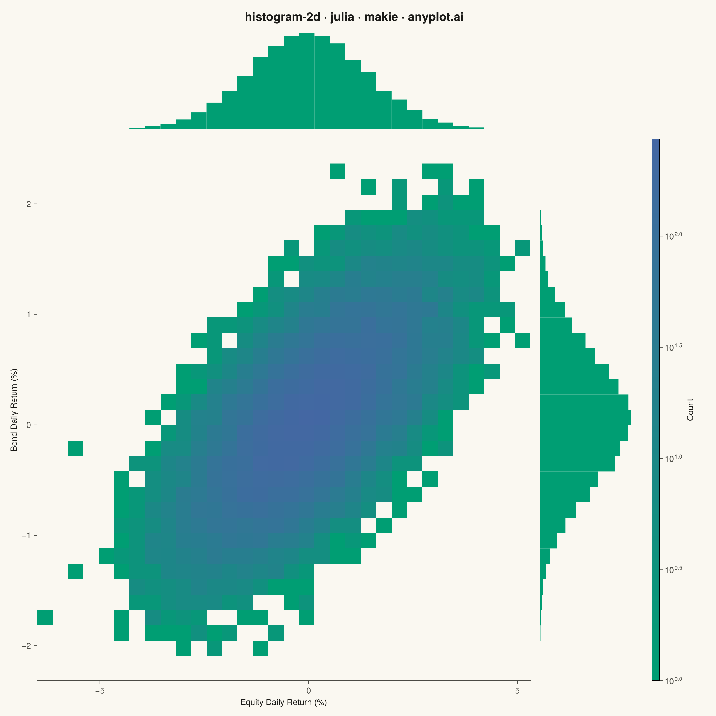
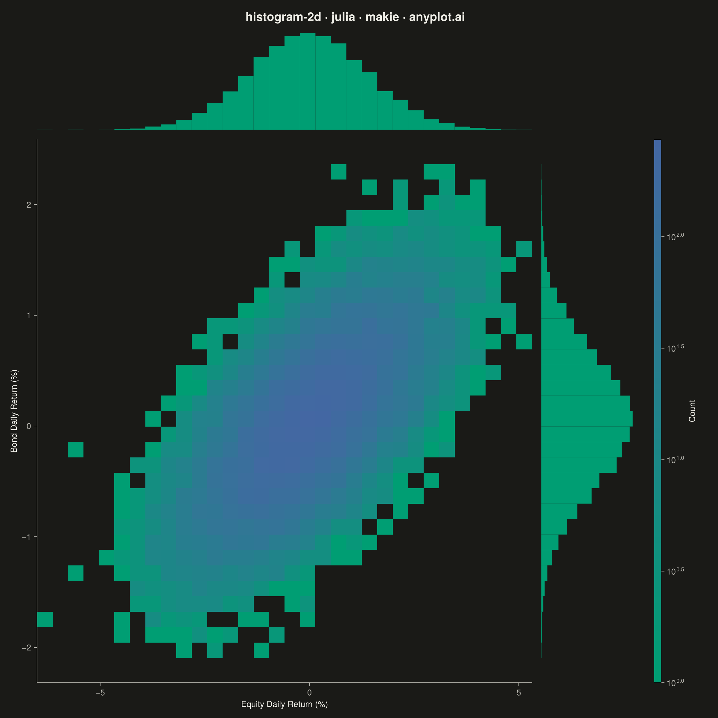
A two-dimensional histogram that displays the joint distribution of two continuous variables as a heatmap with rectangular bins. Each bin's color intensity represents the frequency or count of data points falling within that region, making it ideal for revealing density patterns, clusters, and correlations in bivariate data. Unlike scatter plots that can become cluttered with large datasets, 2D histograms effectively summarize point density.
# anyplot.ai
# histogram-2d: 2D Histogram Heatmap
# Library: makie 0.21.9 | Julia 1.11.9
# Quality: 91/100 | Created: 2026-09-05

using CairoMakie
using Colors
using ColorSchemes
using Random

Random.seed!(42)

# Theme tokens
const THEME    = get(ENV, "ANYPLOT_THEME", "light")
const PAGE_BG  = THEME == "light" ? colorant"#FAF8F1" : colorant"#1A1A17"
const INK      = THEME == "light" ? colorant"#1A1A17" : colorant"#F0EFE8"
const INK_SOFT = THEME == "light" ? colorant"#4A4A44" : colorant"#B8B7B0"
const IMPRINT_PALETTE = [
    colorant"#009E73", colorant"#C475FD", colorant"#4467A3", colorant"#BD8233",
    colorant"#AE3030", colorant"#2ABCCD", colorant"#954477", colorant"#99B314",
]
const IMPRINT_SEQ = cgrad([colorant"#009E73", colorant"#4467A3"])

# Data — correlated daily returns for two asset classes (%)
n_points = 20_000
correlation = 0.65
z1 = randn(n_points)
z2 = randn(n_points)
equity_returns = z1 .* 1.4
bond_returns = (correlation .* z1 .+ sqrt(1 - correlation^2) .* z2) .* 0.6 .+ 0.05

# 2D histogram binning (rectangular bins)
n_bins = 32
x_edges = range(minimum(equity_returns), maximum(equity_returns), length = n_bins + 1)
y_edges = range(minimum(bond_returns), maximum(bond_returns), length = n_bins + 1)
counts = zeros(Int, n_bins, n_bins)
for i in eachindex(equity_returns)
    xi = clamp(searchsortedlast(x_edges, equity_returns[i]), 1, n_bins)
    yi = clamp(searchsortedlast(y_edges, bond_returns[i]), 1, n_bins)
    counts[xi, yi] += 1
end
x_centers = (x_edges[1:end-1] .+ x_edges[2:end]) ./ 2
y_centers = (y_edges[1:end-1] .+ y_edges[2:end]) ./ 2

# Empty bins render as page background instead of the colormap's low end,
# so the density shape stands out instead of a solid-green rectangle
counts_display = Float64.(counts)
counts_display[counts_display .== 0] .= NaN

# Plot — joint density heatmap with marginal histograms for univariate context
title_str = "histogram-2d · julia · makie · anyplot.ai"

fig = Figure(resolution = (1200, 1200), fontsize = 14, backgroundcolor = PAGE_BG)

Label(fig[1, 1:3], title_str; fontsize = 20, color = INK, font = :bold)

ax_top = Axis(fig[2, 1]; backgroundcolor = PAGE_BG)

ax_main = Axis(
    fig[3, 1];
    xlabel = "Equity Daily Return (%)",
    ylabel = "Bond Daily Return (%)",
    xlabelcolor = INK,
    ylabelcolor = INK,
    xticklabelcolor = INK_SOFT,
    yticklabelcolor = INK_SOFT,
    xtickcolor = INK_SOFT,
    ytickcolor = INK_SOFT,
    backgroundcolor = PAGE_BG,
    topspinevisible = false,
    rightspinevisible = false,
    leftspinecolor = INK_SOFT,
    bottomspinecolor = INK_SOFT,
    xgridvisible = false,
    ygridvisible = false,
    xlabelsize = 14,
    ylabelsize = 14,
    xticklabelsize = 14,
    yticklabelsize = 14,
)

ax_right = Axis(fig[3, 2]; backgroundcolor = PAGE_BG)

linkxaxes!(ax_top, ax_main)
linkyaxes!(ax_right, ax_main)

hist!(ax_top, equity_returns; bins = x_edges, color = IMPRINT_PALETTE[1])
# Log color scale reveals structure in the sparse outer lobes (counts span ~1 to 170+)
hm = heatmap!(
    ax_main,
    x_centers,
    y_centers,
    counts_display;
    colormap = IMPRINT_SEQ,
    nan_color = PAGE_BG,
    colorscale = log10,
)
hist!(ax_right, bond_returns; bins = y_edges, direction = :x, color = IMPRINT_PALETTE[1])

hidedecorations!(ax_top)
hidespines!(ax_top)
hidedecorations!(ax_right)
hidespines!(ax_right)

Colorbar(
    fig[3, 3],
    hm;
    label = "Count",
    labelcolor = INK,
    ticklabelcolor = INK_SOFT,
    tickcolor = INK_SOFT,
    labelsize = 14,
    ticklabelsize = 14,
)

rowsize!(fig.layout, 2, Relative(0.16))
colsize!(fig.layout, 2, Relative(0.16))
colsize!(fig.layout, 3, Relative(0.05))
rowgap!(fig.layout, 8)
colgap!(fig.layout, 8)

# Save
save("plot-$(THEME).png", fig; px_per_unit = 2)
Runnable source as JSON, for any HTTP client: https://api.anyplot.ai/specs/histogram-2d/makie/code. Any spec id and library id listed in llms-full.txt fit the same URL shape; every URL below is complete and callable.
{
  "spec_id": "histogram-2d",
  "language": "julia",
  "library": "makie",
  "page": "https://anyplot.ai/histogram-2d/julia/makie",
  "hub": "https://anyplot.ai/histogram-2d",
  "code_json": "https://api.anyplot.ai/specs/histogram-2d/makie/code",
  "spec_json": "https://api.anyplot.ai/specs/histogram-2d",
  "render_light_png": "https://storage.googleapis.com/anyplot-images/plots/histogram-2d/julia/makie/plot-light.png",
  "render_dark_png": "https://storage.googleapis.com/anyplot-images/plots/histogram-2d/julia/makie/plot-dark.png",
  "quality_score": 91.0,
  "license": "MIT",
  "guide": "https://anyplot.ai/llms.txt"
}
Part of 2D Histogram Heatmap on anyplot.ai.