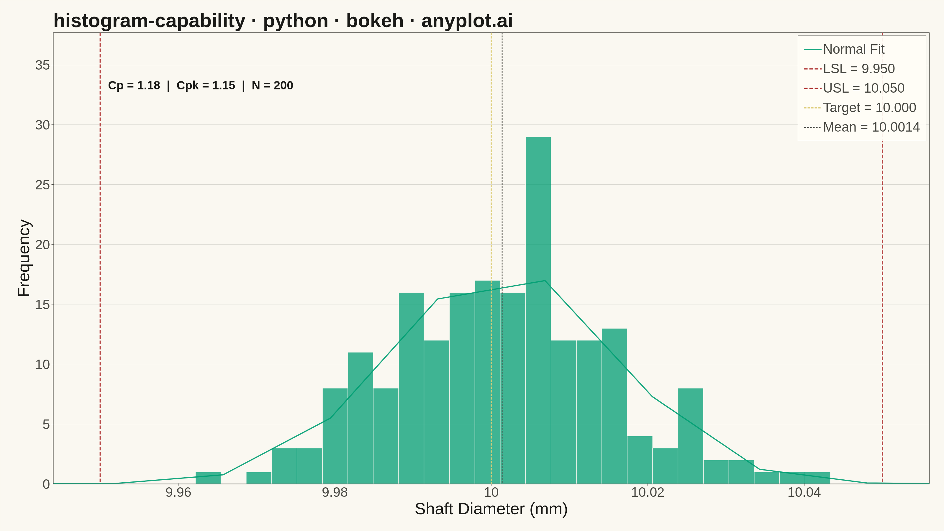
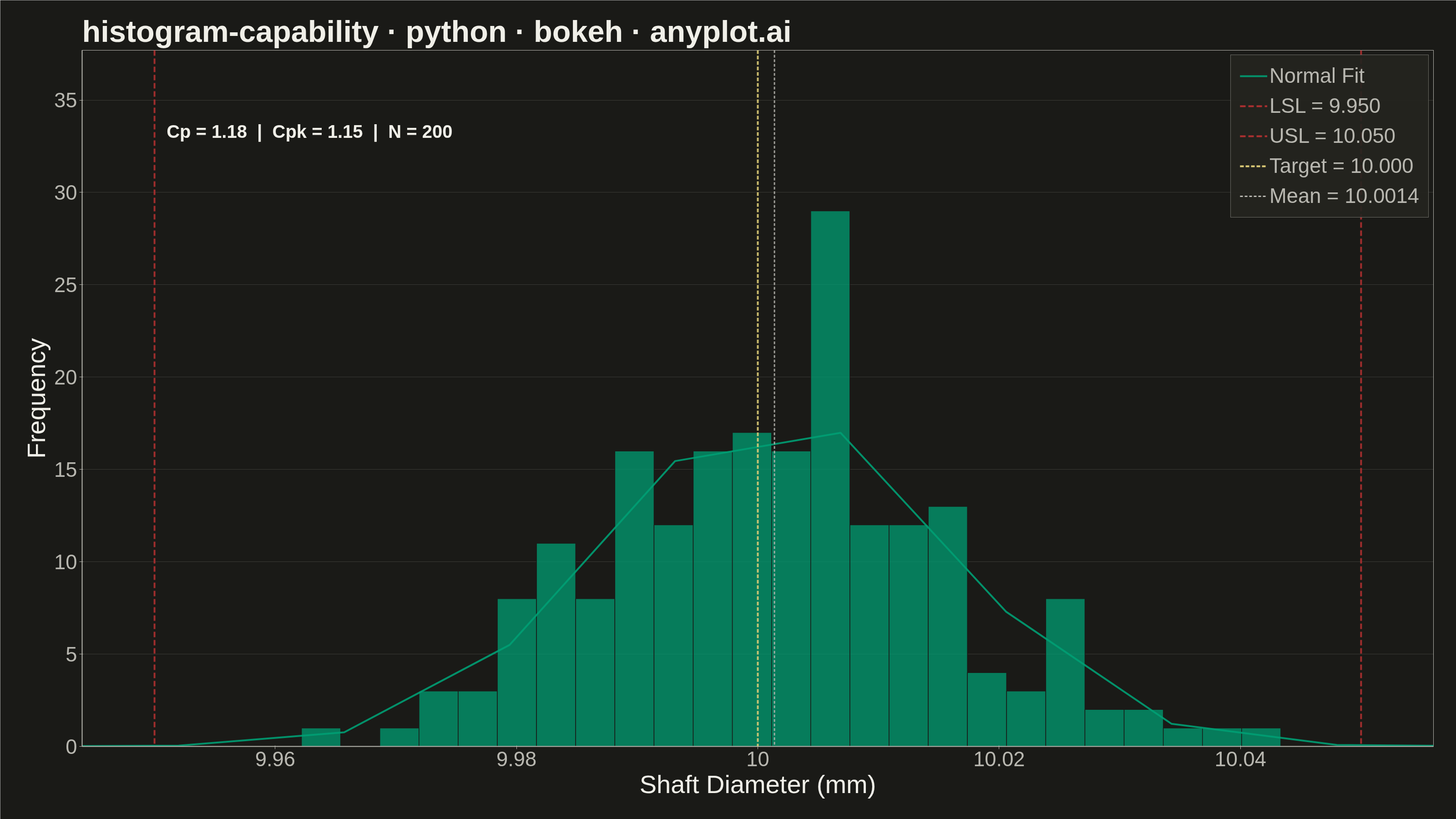
A process capability plot displays a histogram of measured process data overlaid with a fitted normal distribution curve and vertical lines for specification limits (LSL, USL) and target value. Capability indices (Cp, Cpk) are annotated on the plot to quantify how well the process meets specifications. This is a standard tool in quality engineering and Six Sigma for assessing whether a manufacturing or production process is capable of consistently producing output within tolerance.
""" anyplot.ai
histogram-capability: Process Capability Plot with Specification Limits
Library: bokeh 3.9.1 | Python 3.13.14
Quality: 89/100 | Updated: 2026-06-20
"""

import os
import sys


# Remove this file's own directory from sys.path so 'import bokeh' resolves
# to the installed package, not this file.
_here = os.path.dirname(os.path.abspath(__file__))
sys.path = [p for p in sys.path if os.path.abspath(p or ".") != _here]

import time
from pathlib import Path

import numpy as np
from bokeh.io import output_file, save
from bokeh.models import ColumnDataSource, HoverTool, Label, Legend, LegendItem, Span
from bokeh.plotting import figure
from scipy import stats
from selenium import webdriver
from selenium.webdriver.chrome.options import Options


THEME = os.getenv("ANYPLOT_THEME", "light")

# Imprint palette — theme-adaptive chrome tokens
PAGE_BG = "#FAF8F1" if THEME == "light" else "#1A1A17"
ELEVATED_BG = "#FFFDF6" if THEME == "light" else "#242420"
INK = "#1A1A17" if THEME == "light" else "#F0EFE8"
INK_SOFT = "#4A4A44" if THEME == "light" else "#B8B7B0"
INK_MUTED = "#6B6A63" if THEME == "light" else "#A8A79F"

# Imprint categorical palette (8 hues, hybrid-v3 sort order)
IMPRINT_PALETTE = ["#009E73", "#C475FD", "#4467A3", "#BD8233", "#AE3030", "#2ABCCD", "#954477", "#99B314"]
ANYPLOT_AMBER = "#DDCC77"  # warning / caution anchor

# Data — machined shaft diameter (mm)
# Barely-capable process (Cp ~1.10, Cpk ~1.05) with sigma wide enough that
# the distribution fills the spec window and tails approach both LSL and USL.
np.random.seed(42)
lsl = 9.950
usl = 10.050
target = 10.000
measurements = np.random.normal(loc=10.002, scale=0.0152, size=200)

# Statistics
mean_val = np.mean(measurements)
sigma = np.std(measurements, ddof=1)
cp = (usl - lsl) / (6 * sigma)
cpk = min((usl - mean_val) / (3 * sigma), (mean_val - lsl) / (3 * sigma))

# Histogram bins
counts, edges = np.histogram(measurements, bins=25)
left_edges = edges[:-1]
right_edges = edges[1:]
max_count = counts.max()

source = ColumnDataSource(
    data={
        "left": left_edges,
        "right": right_edges,
        "top": counts,
        "bottom": [0] * len(counts),
        "count": counts,
        "bin_start": [f"{e:.4f}" for e in left_edges],
        "bin_end": [f"{e:.4f}" for e in right_edges],
    }
)

# Normal distribution curve
x_min = min(lsl - 2.0, measurements.min() - 0.5)
x_max = max(usl + 2.0, measurements.max() + 0.5)
x_curve = np.linspace(x_min, x_max, 300)
bin_width = edges[1] - edges[0]
y_curve = stats.norm.pdf(x_curve, mean_val, sigma) * len(measurements) * bin_width
curve_source = ColumnDataSource(data={"x": x_curve, "y": y_curve})

# Create figure — canonical 3200×1800 landscape canvas
p = figure(
    width=3200,
    height=1800,
    title="histogram-capability · python · bokeh · anyplot.ai",
    x_axis_label="Shaft Diameter (mm)",
    y_axis_label="Frequency",
    toolbar_location=None,
    min_border_bottom=160,
    min_border_left=180,
    min_border_top=110,
    min_border_right=50,
)

# Histogram bars — Imprint green (#009E73) is always first series
bars = p.quad(
    left="left",
    right="right",
    top="top",
    bottom="bottom",
    source=source,
    fill_color=IMPRINT_PALETTE[0],
    fill_alpha=0.75,
    line_color=PAGE_BG,
    line_width=1.5,
    hover_fill_color=IMPRINT_PALETTE[3],  # ochre hover highlight
    hover_fill_alpha=0.95,
    hover_line_color=PAGE_BG,
)

# Hover tool
hover = HoverTool(renderers=[bars], tooltips=[("Range", "@bin_start – @bin_end mm"), ("Count", "@count")], mode="mouse")
p.add_tools(hover)

# Normal distribution curve — matching Imprint green
curve_line = p.line(x="x", y="y", source=curve_source, line_color=IMPRINT_PALETTE[0], line_width=4, line_alpha=0.9)

# Spec limit lines — matte red (semantic: out-of-spec boundary)
lsl_span = Span(
    location=lsl, dimension="height", line_color=IMPRINT_PALETTE[4], line_width=4, line_dash=[12, 6], line_alpha=0.9
)
usl_span = Span(
    location=usl, dimension="height", line_color=IMPRINT_PALETTE[4], line_width=4, line_dash=[12, 6], line_alpha=0.9
)
p.add_layout(lsl_span)
p.add_layout(usl_span)

# Target line — amber (semantic: nominal / reference)
target_span = Span(
    location=target, dimension="height", line_color=ANYPLOT_AMBER, line_width=4, line_dash=[8, 4], line_alpha=0.9
)
p.add_layout(target_span)

# Mean line — theme-adaptive ink (structural / metadata layer)
mean_span = Span(
    location=mean_val, dimension="height", line_color=INK_SOFT, line_width=3, line_dash=[6, 4], line_alpha=0.85
)
p.add_layout(mean_span)

# Off-screen renderers so Span objects appear in the legend
_off = -9999
lsl_legend_line = p.line(x=[_off, _off], y=[_off, _off], line_color=IMPRINT_PALETTE[4], line_width=4, line_dash=[12, 6])
usl_legend_line = p.line(x=[_off, _off], y=[_off, _off], line_color=IMPRINT_PALETTE[4], line_width=4, line_dash=[12, 6])
target_legend_line = p.line(x=[_off, _off], y=[_off, _off], line_color=ANYPLOT_AMBER, line_width=4, line_dash=[8, 4])
mean_legend_line = p.line(x=[_off, _off], y=[_off, _off], line_color=INK_SOFT, line_width=3, line_dash=[6, 4])

# Legend
legend = Legend(
    items=[
        LegendItem(label="Normal Fit", renderers=[curve_line]),
        LegendItem(label=f"LSL = {lsl:.3f}", renderers=[lsl_legend_line]),
        LegendItem(label=f"USL = {usl:.3f}", renderers=[usl_legend_line]),
        LegendItem(label=f"Target = {target:.3f}", renderers=[target_legend_line]),
        LegendItem(label=f"Mean = {mean_val:.4f}", renderers=[mean_legend_line]),
    ],
    location="top_right",
    label_text_font_size="34pt",
    label_text_color=INK_SOFT,
    glyph_width=60,
    glyph_height=6,
    spacing=14,
    padding=20,
    background_fill_alpha=0.92,
    background_fill_color=ELEVATED_BG,
    border_line_color=INK_SOFT,
    border_line_alpha=0.5,
)
p.add_layout(legend, "center")

# Capability indices annotation
cap_text = f"Cp = {cp:.2f}  |  Cpk = {cpk:.2f}  |  N = {len(measurements)}"
cap_label = Label(
    x=lsl + 0.001, y=max_count * 1.13, text=cap_text, text_font_size="30pt", text_color=INK, text_font_style="bold"
)
p.add_layout(cap_label)

# Typography — canonical bokeh sizes for 3200×1800
p.title.text_font_size = "50pt"
p.title.text_color = INK
p.title.text_font_style = "bold"
p.xaxis.axis_label_text_font_size = "42pt"
p.yaxis.axis_label_text_font_size = "42pt"
p.xaxis.axis_label_text_color = INK
p.xaxis.axis_label_text_font_style = "normal"
p.yaxis.axis_label_text_color = INK
p.yaxis.axis_label_text_font_style = "normal"
p.xaxis.major_label_text_font_size = "34pt"
p.yaxis.major_label_text_font_size = "34pt"
p.xaxis.major_label_text_color = INK_SOFT
p.yaxis.major_label_text_color = INK_SOFT

# Grid — y-axis only, subtle
p.xgrid.visible = False
p.ygrid.grid_line_alpha = 0.15
p.ygrid.grid_line_color = INK
p.ygrid.grid_line_width = 1

# Chrome — theme-adaptive
p.outline_line_color = INK_SOFT
p.background_fill_color = PAGE_BG
p.border_fill_color = PAGE_BG
p.xaxis.axis_line_width = 2
p.yaxis.axis_line_width = 2
p.xaxis.axis_line_color = INK_SOFT
p.yaxis.axis_line_color = INK_SOFT
p.xaxis.minor_tick_line_color = None
p.yaxis.minor_tick_line_color = None
p.xaxis.major_tick_line_color = INK_SOFT
p.yaxis.major_tick_line_color = INK_SOFT

# Axis ranges — tightened to avoid empty space at edges
data_min = measurements.min()
data_max = measurements.max()
spec_min = min(lsl, data_min)
spec_max = max(usl, data_max)
edge_margin = (spec_max - spec_min) * 0.06
p.x_range.start = spec_min - edge_margin
p.x_range.end = spec_max + edge_margin
p.y_range.start = 0
p.y_range.end = max_count * 1.30

# Save interactive HTML artifact
output_file(f"plot-{THEME}.html")
save(p)

# Screenshot via headless Chrome — Selenium 4 auto-resolves chromedriver.
# Use CDP captureScreenshot with captureBeyondViewport=True so the full
# 3200×1800 Bokeh canvas is captured even when Chrome's inner viewport is
# smaller than the outer window-size (headless Chrome reserves ~143px for
# virtual browser chrome that shrinks innerHeight below the window height).
import base64


W, H = 3200, 1800
opts = Options()
for arg in (
    "--headless=new",
    "--no-sandbox",
    "--disable-dev-shm-usage",
    "--disable-gpu",
    f"--window-size={W},{H}",
    "--hide-scrollbars",
):
    opts.add_argument(arg)
driver = webdriver.Chrome(options=opts)
driver.set_window_size(W, H)
driver.get(f"file://{Path(f'plot-{THEME}.html').resolve()}")
time.sleep(3)
result = driver.execute_cdp_cmd(
    "Page.captureScreenshot",
    {"format": "png", "clip": {"x": 0, "y": 0, "width": W, "height": H, "scale": 1}, "captureBeyondViewport": True},
)
with open(f"plot-{THEME}.png", "wb") as f:
    f.write(base64.b64decode(result["data"]))
driver.quit()
Runnable source as JSON, for any HTTP client: https://api.anyplot.ai/specs/histogram-capability/bokeh/code. Any spec id and library id listed in llms-full.txt fit the same URL shape; every URL below is complete and callable.
{
  "spec_id": "histogram-capability",
  "language": "python",
  "library": "bokeh",
  "page": "https://anyplot.ai/histogram-capability/python/bokeh",
  "hub": "https://anyplot.ai/histogram-capability",
  "code_json": "https://api.anyplot.ai/specs/histogram-capability/bokeh/code",
  "spec_json": "https://api.anyplot.ai/specs/histogram-capability",
  "render_light_png": "https://storage.googleapis.com/anyplot-images/plots/histogram-capability/python/bokeh/plot-light.png",
  "render_dark_png": "https://storage.googleapis.com/anyplot-images/plots/histogram-capability/python/bokeh/plot-dark.png",
  "interactive_light_html": "https://storage.googleapis.com/anyplot-images/plots/histogram-capability/python/bokeh/plot-light.html",
  "interactive_dark_html": "https://storage.googleapis.com/anyplot-images/plots/histogram-capability/python/bokeh/plot-dark.html",
  "quality_score": 89.0,
  "license": "MIT",
  "guide": "https://anyplot.ai/llms.txt"
}
Part of Process Capability Plot with Specification Limits on anyplot.ai.