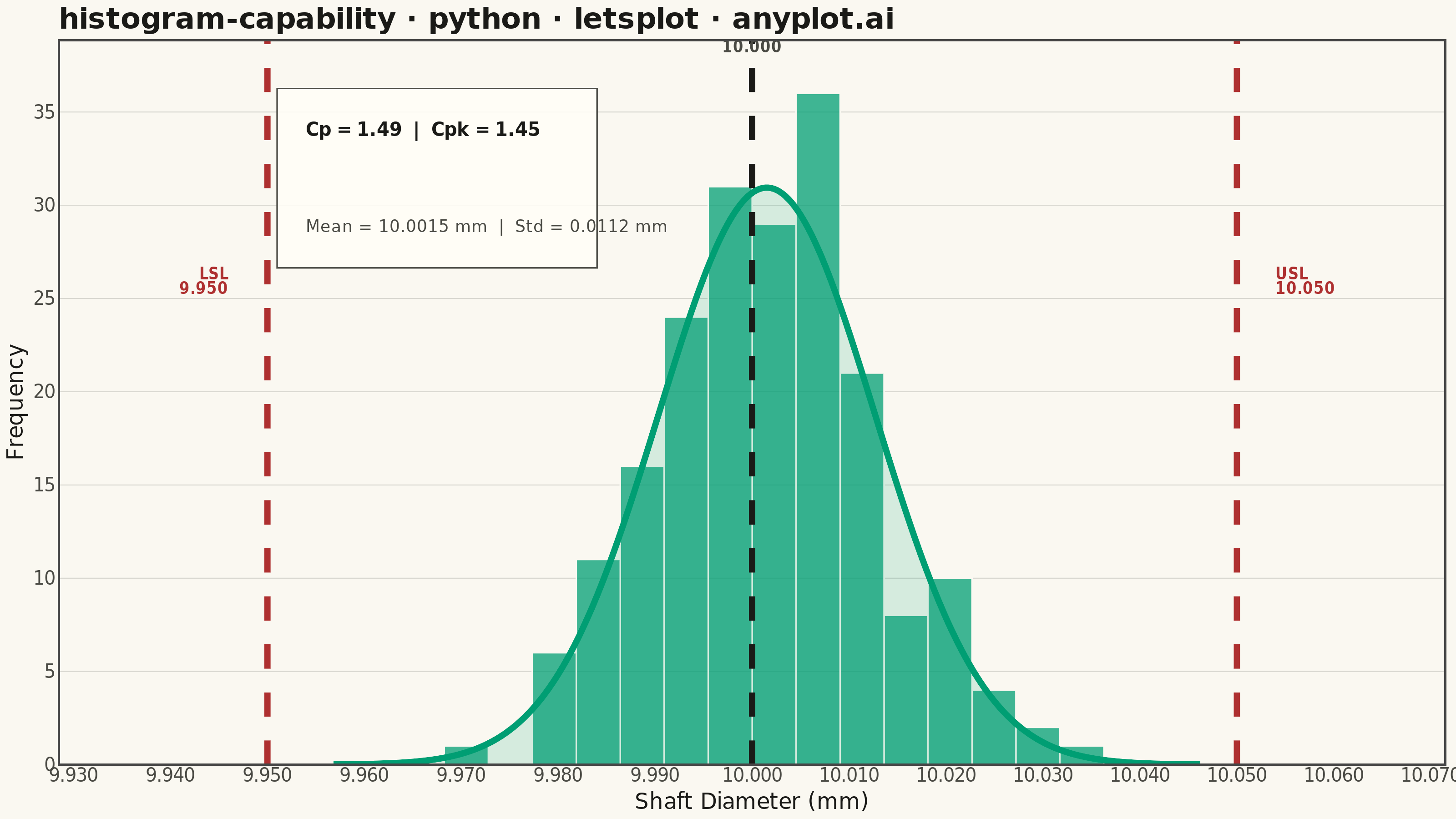
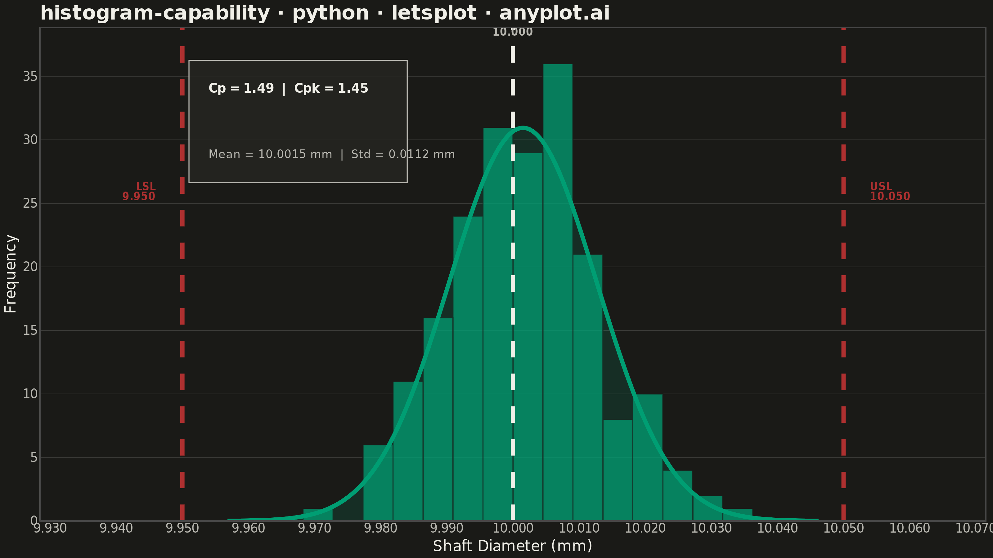
A process capability plot displays a histogram of measured process data overlaid with a fitted normal distribution curve and vertical lines for specification limits (LSL, USL) and target value. Capability indices (Cp, Cpk) are annotated on the plot to quantify how well the process meets specifications. This is a standard tool in quality engineering and Six Sigma for assessing whether a manufacturing or production process is capable of consistently producing output within tolerance.
""" anyplot.ai
histogram-capability: Process Capability Plot with Specification Limits
Library: letsplot 4.10.1 | Python 3.13.14
Quality: 89/100 | Updated: 2026-06-20
"""

import os

import numpy as np
import pandas as pd
from lets_plot import (
    LetsPlot,
    aes,
    element_blank,
    element_line,
    element_rect,
    element_text,
    geom_area,
    geom_histogram,
    geom_rect,
    geom_text,
    geom_vline,
    ggplot,
    ggsize,
    labs,
    layer_tooltips,
    scale_x_continuous,
    scale_y_continuous,
    theme,
    theme_minimal,
)
from lets_plot.export import ggsave
from scipy import stats


LetsPlot.setup_html()

# Theme tokens — Imprint palette, theme-adaptive chrome
THEME = os.getenv("ANYPLOT_THEME", "light")
PAGE_BG = "#FAF8F1" if THEME == "light" else "#1A1A17"
INK = "#1A1A17" if THEME == "light" else "#F0EFE8"
INK_SOFT = "#4A4A44" if THEME == "light" else "#B8B7B0"
# Pre-blended grid color: 15% INK over PAGE_BG (rgba() avoids dependency on CSS parser)
GRID_COLOR = "#D8D7D0" if THEME == "light" else "#3A3A37"
ELEVATED_BG = "#FFFDF6" if THEME == "light" else "#242420"

IMPRINT_PALETTE = ["#009E73", "#C475FD", "#4467A3", "#BD8233", "#AE3030", "#2ABCCD", "#954477", "#99B314"]
BRAND = IMPRINT_PALETTE[0]  # #009E73 — always first series (histogram bars + curve)
LIMIT_COLOR = IMPRINT_PALETTE[4]  # #AE3030 — matte red, semantic: out-of-spec danger

# Data — shaft diameter measurements (mm), Six Sigma precision machining
np.random.seed(42)
lsl = 9.95
usl = 10.05
target = 10.00
margin = 0.015

measurements = np.random.normal(loc=10.002, scale=0.012, size=200)
sample_mean = float(np.mean(measurements))
sample_std = float(np.std(measurements, ddof=1))

# Capability indices per Six Sigma formulas
cp = (usl - lsl) / (6 * sample_std)
cpk = min((usl - sample_mean) / (3 * sample_std), (sample_mean - lsl) / (3 * sample_std))

df = pd.DataFrame({"measurement": measurements})

# Compute bins matching lets-plot's geom_histogram(bins=30) behavior:
# lets-plot bins the data over the visible x range (limits from scale_x_continuous)
lp_bins = np.linspace(lsl - margin, usl + margin, 31)
hist_counts, _ = np.histogram(measurements, bins=lp_bins)
y_max = float(hist_counts.max())
lp_bin_width = float(lp_bins[1] - lp_bins[0])

# Normal distribution curve fitted to sample mean and std
x_curve = np.linspace(sample_mean - 4 * sample_std, sample_mean + 4 * sample_std, 300)
y_curve = stats.norm.pdf(x_curve, sample_mean, sample_std)
y_curve_scaled = y_curve * lp_bin_width * len(measurements)
df_curve = pd.DataFrame({"x": x_curve, "y": y_curve_scaled})

cap_text = f"Cp = {cp:.2f}  |  Cpk = {cpk:.2f}"
stats_text = f"Mean = {sample_mean:.4f} mm  |  Std = {sample_std:.4f} mm"

# Place capability text in upper-left tail region (above low-count bars)
ann_x = lsl + 0.004
ann_df = pd.DataFrame({"x": [ann_x], "y": [y_max * 0.92], "label": [cap_text]})
stats_ann_df = pd.DataFrame({"x": [ann_x], "y": [y_max * 0.78], "label": [stats_text]})

# Spec limit labels — symmetric margins, labels outside bars
lsl_label_df = pd.DataFrame({"x": [lsl - 0.004], "y": [y_max * 0.70], "label": ["LSL\n9.950"]})
usl_label_df = pd.DataFrame({"x": [usl + 0.004], "y": [y_max * 0.70], "label": ["USL\n10.050"]})
# Target label above histogram top (clear of bars and curve)
target_label_df = pd.DataFrame({"x": [target], "y": [y_max * 1.05], "label": ["Target\n10.000"]})

# Title (53 chars < 67 baseline, no scaling needed)
title = "histogram-capability · python · letsplot · anyplot.ai"

# Plot
plot = (
    ggplot(df, aes(x="measurement"))
    + geom_histogram(
        bins=30,
        fill=BRAND,
        color=PAGE_BG,
        alpha=0.75,
        size=0.3,
        tooltips=layer_tooltips().format("..count..", "d").line("Count|@..count.."),
    )
    + geom_area(
        data=df_curve, mapping=aes(x="x", y="y"), fill=BRAND, alpha=0.15, color=BRAND, size=1.5, inherit_aes=False
    )
    # Specification limits: matte red = out-of-spec semantic anchor
    + geom_vline(xintercept=lsl, color=LIMIT_COLOR, size=1.5, linetype="dashed")
    + geom_vline(xintercept=usl, color=LIMIT_COLOR, size=1.5, linetype="dashed")
    # Target: INK neutral = reference/baseline semantic anchor (theme-adaptive)
    + geom_vline(xintercept=target, color=INK, size=1.5, linetype="dashed")
    + geom_text(
        data=lsl_label_df,
        mapping=aes(x="x", y="y", label="label"),
        size=4,
        color=LIMIT_COLOR,
        fontface="bold",
        hjust=1,
        inherit_aes=False,
    )
    + geom_text(
        data=usl_label_df,
        mapping=aes(x="x", y="y", label="label"),
        size=4,
        color=LIMIT_COLOR,
        fontface="bold",
        hjust=0,
        inherit_aes=False,
    )
    + geom_text(
        data=target_label_df,
        mapping=aes(x="x", y="y", label="label"),
        size=4,
        color=INK_SOFT,
        fontface="bold",
        hjust=0.5,
        inherit_aes=False,
    )
    # Subtle callout box behind capability indices for visual anchoring
    + geom_rect(
        xmin=ann_x - 0.003,
        xmax=ann_x + 0.030,
        ymin=y_max * 0.72,
        ymax=y_max * 0.98,
        fill=ELEVATED_BG,
        color=INK_SOFT,
        alpha=0.90,
        size=0.3,
        inherit_aes=False,
    )
    # Capability indices — most prominent annotation
    + geom_text(
        data=ann_df,
        mapping=aes(x="x", y="y", label="label"),
        size=5,
        color=INK,
        fontface="bold",
        hjust=0,
        inherit_aes=False,
    )
    + geom_text(
        data=stats_ann_df,
        mapping=aes(x="x", y="y", label="label"),
        size=4.5,
        color=INK_SOFT,
        hjust=0,
        inherit_aes=False,
    )
    + scale_x_continuous(name="Shaft Diameter (mm)", format=".3f", limits=[lsl - margin, usl + margin])
    + scale_y_continuous(name="Frequency", format="d", expand=[0, 0, 0.15, 0])
    + labs(title=title)
    + theme_minimal()
    + theme(
        plot_title=element_text(size=16, face="bold", color=INK),
        axis_title=element_text(size=12, color=INK),
        axis_text=element_text(size=10, color=INK_SOFT),
        legend_position="none",
        panel_grid_major_x=element_blank(),
        panel_grid_minor=element_blank(),
        panel_grid_major_y=element_line(color=GRID_COLOR, size=0.5),
        plot_background=element_rect(fill=PAGE_BG, color=PAGE_BG),
        panel_background=element_rect(fill=PAGE_BG),
        axis_line=element_line(color=INK_SOFT),
    )
    + ggsize(800, 450)
)

# Save
ggsave(plot, f"plot-{THEME}.png", path=".", scale=4)
ggsave(plot, f"plot-{THEME}.html", path=".")
Runnable source as JSON, for any HTTP client: https://api.anyplot.ai/specs/histogram-capability/letsplot/code. Any spec id and library id listed in llms-full.txt fit the same URL shape; every URL below is complete and callable.
{
  "spec_id": "histogram-capability",
  "language": "python",
  "library": "letsplot",
  "page": "https://anyplot.ai/histogram-capability/python/letsplot",
  "hub": "https://anyplot.ai/histogram-capability",
  "code_json": "https://api.anyplot.ai/specs/histogram-capability/letsplot/code",
  "spec_json": "https://api.anyplot.ai/specs/histogram-capability",
  "render_light_png": "https://storage.googleapis.com/anyplot-images/plots/histogram-capability/python/letsplot/plot-light.png",
  "render_dark_png": "https://storage.googleapis.com/anyplot-images/plots/histogram-capability/python/letsplot/plot-dark.png",
  "interactive_light_html": "https://storage.googleapis.com/anyplot-images/plots/histogram-capability/python/letsplot/plot-light.html",
  "interactive_dark_html": "https://storage.googleapis.com/anyplot-images/plots/histogram-capability/python/letsplot/plot-dark.html",
  "quality_score": 89.0,
  "license": "MIT",
  "guide": "https://anyplot.ai/llms.txt"
}
Part of Process Capability Plot with Specification Limits on anyplot.ai.