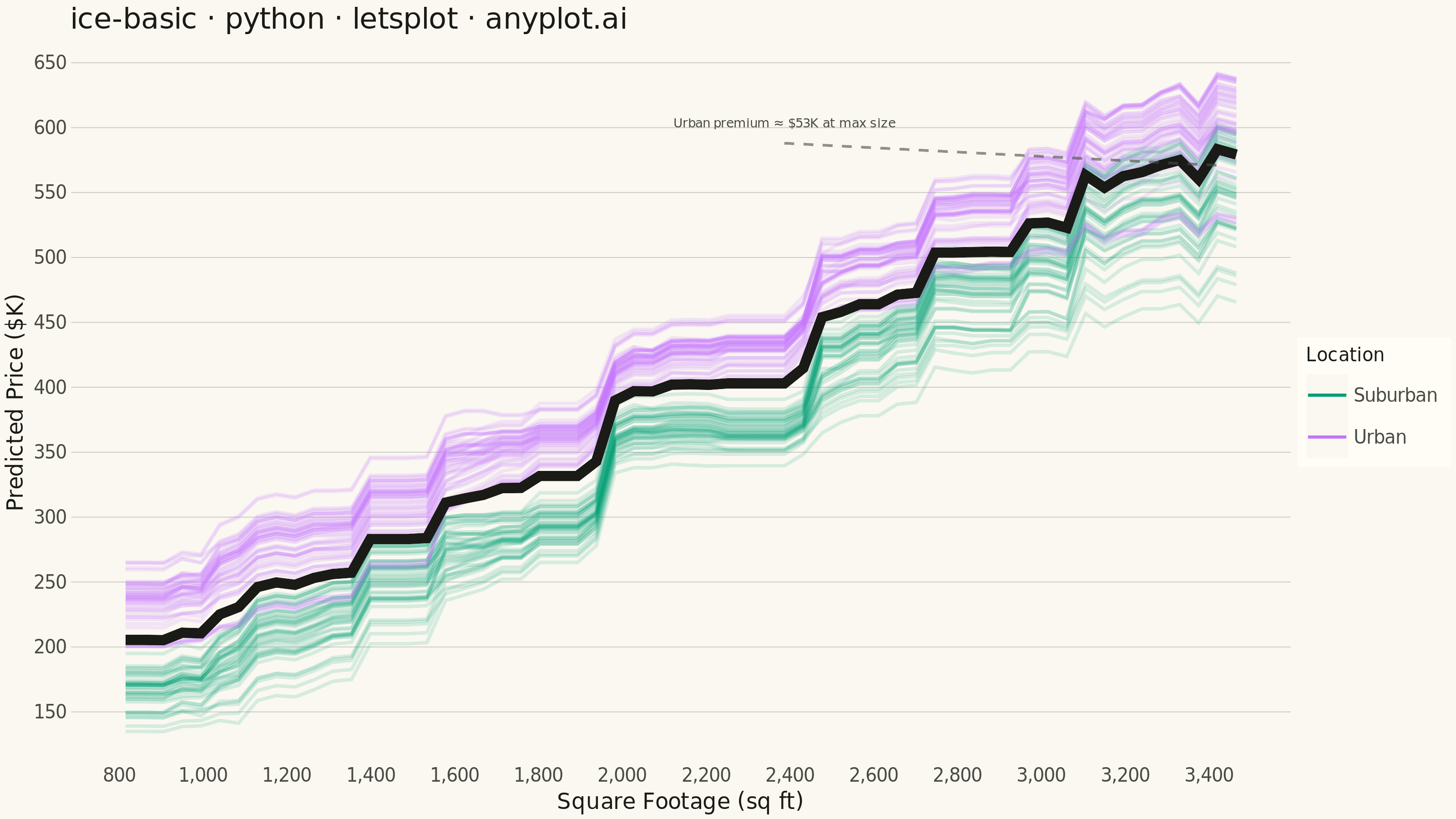
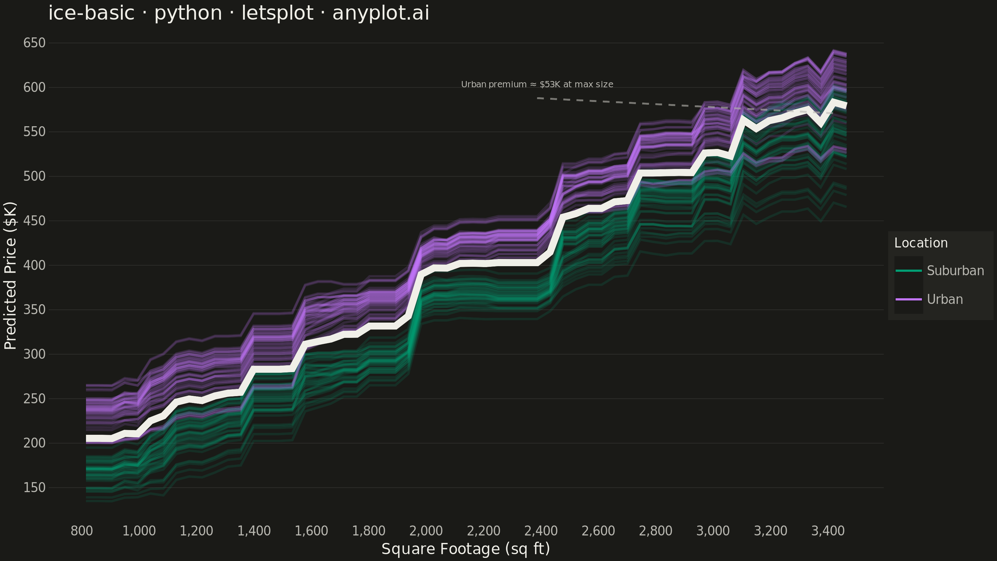
The same plot in 14 other libraries — Python: Altair, Bokeh, Matplotlib, Plotly, plotnine, Pygal, Seaborn; R: ggplot2; Julia: Makie.jl; JavaScript: Chart.js, D3.js, Apache ECharts, Highcharts, MUI X Charts. Compare all 15 side by side: Individual Conditional Expectation (ICE) Plot in Python, R, Julia and JavaScript.
An Individual Conditional Expectation (ICE) plot visualizes how the predicted outcome of a machine learning model changes for each individual observation as a single feature varies across its range. Unlike partial dependence plots (PDP) that show the average marginal effect, ICE plots display one line per observation, revealing heterogeneous effects, feature interactions, and subgroup-specific behaviors that would be hidden by averaging. This makes ICE plots essential for detecting when a feature's effect varies across the population.
""" anyplot.ai
ice-basic: Individual Conditional Expectation (ICE) Plot
Library: letsplot 4.11.0 | Python 3.13.15
Quality: 93/100 | Updated: 2026-08-17
"""

import os

import numpy as np
import pandas as pd
from lets_plot import (
    LetsPlot,
    aes,
    element_blank,
    element_line,
    element_rect,
    element_text,
    geom_line,
    geom_segment,
    geom_text,
    ggplot,
    ggsize,
    labs,
    layer_tooltips,
    scale_color_manual,
    theme,
    theme_minimal,
)
from lets_plot.export import ggsave
from sklearn.ensemble import GradientBoostingRegressor


LetsPlot.setup_html()

# Theme tokens
THEME = os.getenv("ANYPLOT_THEME", "light")
PAGE_BG = "#FAF8F1" if THEME == "light" else "#1A1A17"
ELEVATED_BG = "#FFFDF6" if THEME == "light" else "#242420"
INK = "#1A1A17" if THEME == "light" else "#F0EFE8"
INK_SOFT = "#4A4A44" if THEME == "light" else "#B8B7B0"
GRID_COLOR = "#D0CEC7" if THEME == "light" else "#2E2E2B"

BRAND = "#009E73"  # Imprint palette position 1 — Suburban houses
COLOR2 = "#C475FD"  # Imprint palette position 2 — Urban houses

# Data — house price predictions via GradientBoostingRegressor
np.random.seed(42)
n_obs = 100

sqft = np.random.uniform(800, 3500, n_obs)
bedrooms = np.random.randint(2, 6, n_obs).astype(float)
age = np.random.uniform(1, 50, n_obs)
neighborhood = np.random.choice([0, 1], n_obs)

price = sqft * 150 + bedrooms * 12000 - age * 600 + neighborhood * 75000 + np.random.normal(0, 18000, n_obs)

X = np.column_stack([sqft, bedrooms, age, neighborhood])
model = GradientBoostingRegressor(n_estimators=150, max_depth=3, random_state=42)
model.fit(X, price)

sqft_grid = np.linspace(sqft.min(), sqft.max(), 60)

# ICE curves — one line per observation
ice_rows = []
for i in range(n_obs):
    for sq in sqft_grid:
        X_mod = np.array([[sq, bedrooms[i], age[i], neighborhood[i]]])
        pred = model.predict(X_mod)[0] / 1000
        ice_rows.append(
            {
                "sqft": sq,
                "prediction": pred,
                "obs_id": str(i),
                "location": "Urban" if neighborhood[i] == 1 else "Suburban",
            }
        )

ice_df = pd.DataFrame(ice_rows)

# Partial dependence — average prediction across all observations
pdp_rows = []
for sq in sqft_grid:
    X_mod = X.copy()
    X_mod[:, 0] = sq
    pdp_rows.append({"sqft": sq, "prediction": model.predict(X_mod).mean() / 1000})

pdp_df = pd.DataFrame(pdp_rows)

# Annotation — quantify the neighborhood divergence at the top of the sqft range,
# calling out the interaction effect the color-coding is meant to reveal.
# The callout text sits in the open space above the mid-range bands; a dashed
# leader points at the actual gap so it never overlaps the dense ICE lines.
top_grid = sqft_grid[-5:]
mask_top = ice_df["sqft"].isin(top_grid)
urban_top = ice_df.loc[mask_top & (ice_df["location"] == "Urban"), "prediction"].mean()
suburban_top = ice_df.loc[mask_top & (ice_df["location"] == "Suburban"), "prediction"].mean()
gap_x = sqft_grid[-1]
gap_y = (urban_top + suburban_top) / 2
callout_x = sqft_grid[35]
callout_y = 600.0

gap_label = pd.DataFrame(
    {
        "sqft": [callout_x],
        "prediction": [callout_y],
        "label": [f"Urban premium ≈ ${urban_top - suburban_top:.0f}K at max size"],
    }
)
leader = pd.DataFrame({"x": [callout_x], "y": [callout_y - 12], "xend": [gap_x - 30], "yend": [gap_y]})

# Plot — theme_minimal() drops the panel border entirely (no top/right box);
# a matched panel_background border color keeps it that way after overriding fill
anyplot_theme = theme_minimal() + theme(
    plot_background=element_rect(fill=PAGE_BG, color=PAGE_BG),
    panel_background=element_rect(fill=PAGE_BG, color=PAGE_BG),
    panel_grid_major_y=element_line(color=GRID_COLOR, size=0.5),
    panel_grid_major_x=element_blank(),
    panel_grid_minor=element_blank(),
    axis_title=element_text(color=INK, size=12),
    axis_text=element_text(color=INK_SOFT, size=10),
    plot_title=element_text(color=INK, size=16),
    legend_background=element_rect(fill=ELEVATED_BG, color=INK_SOFT),
    legend_text=element_text(color=INK_SOFT, size=10),
    legend_title=element_text(color=INK, size=10),
)

pdp_tooltips = layer_tooltips().line("Sqft: @sqft").line("Avg. Price: @prediction K")

plot = (
    ggplot()
    + geom_line(
        aes(x="sqft", y="prediction", group="obs_id", color="location"),
        data=ice_df,
        alpha=0.15,
        size=0.8,
        tooltips="none",
    )
    + scale_color_manual(values={"Suburban": BRAND, "Urban": COLOR2})
    + geom_line(aes(x="sqft", y="prediction"), data=pdp_df, color=INK, size=2.5, tooltips=pdp_tooltips)
    + geom_segment(
        aes(x="x", y="y", xend="xend", yend="yend"), data=leader, color=INK_SOFT, size=0.6, alpha=0.6, linetype="dashed"
    )
    + geom_text(
        aes(x="sqft", y="prediction", label="label"), data=gap_label, color=INK_SOFT, size=3.5, hjust=0.5, vjust=0
    )
    + labs(
        x="Square Footage (sq ft)",
        y="Predicted Price ($K)",
        title="ice-basic · python · letsplot · anyplot.ai",
        color="Location",
    )
    + anyplot_theme
    + ggsize(800, 450)
)

# Save
ggsave(plot, filename=f"plot-{THEME}.png", path=".", scale=4)
ggsave(plot, filename=f"plot-{THEME}.html", path=".")
Runnable source as JSON, for any HTTP client: https://api.anyplot.ai/specs/ice-basic/letsplot/code. Any spec id and library id listed in llms-full.txt fit the same URL shape; every URL below is complete and callable.
{
  "spec_id": "ice-basic",
  "language": "python",
  "library": "letsplot",
  "page": "https://anyplot.ai/ice-basic/python/letsplot",
  "hub": "https://anyplot.ai/ice-basic",
  "code_json": "https://api.anyplot.ai/specs/ice-basic/letsplot/code",
  "spec_json": "https://api.anyplot.ai/specs/ice-basic",
  "render_light_png": "https://storage.googleapis.com/anyplot-images/plots/ice-basic/python/letsplot/plot-light.png",
  "render_dark_png": "https://storage.googleapis.com/anyplot-images/plots/ice-basic/python/letsplot/plot-dark.png",
  "interactive_light_html": "https://storage.googleapis.com/anyplot-images/plots/ice-basic/python/letsplot/plot-light.html",
  "interactive_dark_html": "https://storage.googleapis.com/anyplot-images/plots/ice-basic/python/letsplot/plot-dark.html",
  "quality_score": 93.0,
  "license": "MIT",
  "guide": "https://anyplot.ai/llms.txt"
}
Part of Individual Conditional Expectation (ICE) Plot on anyplot.ai.