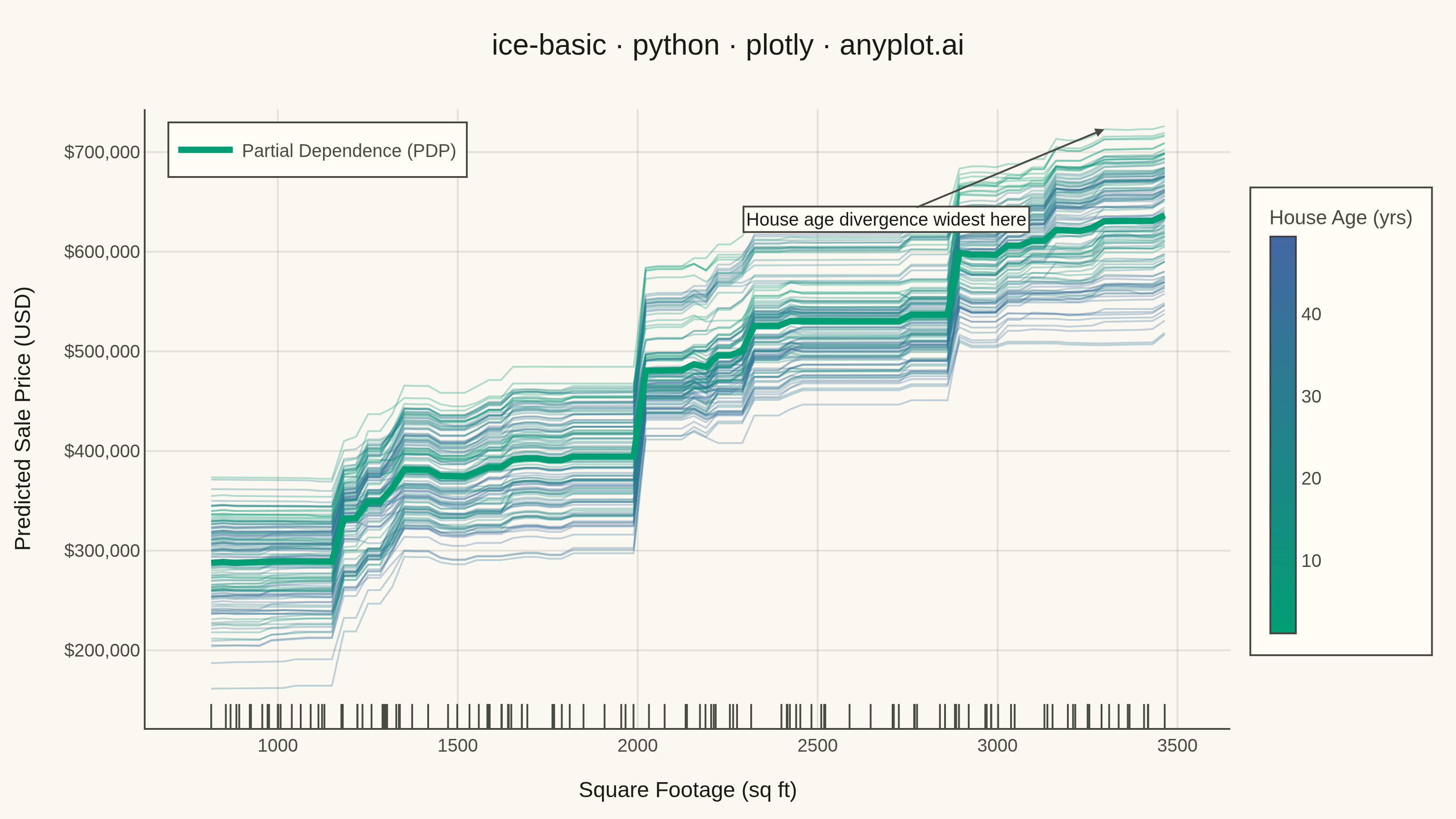
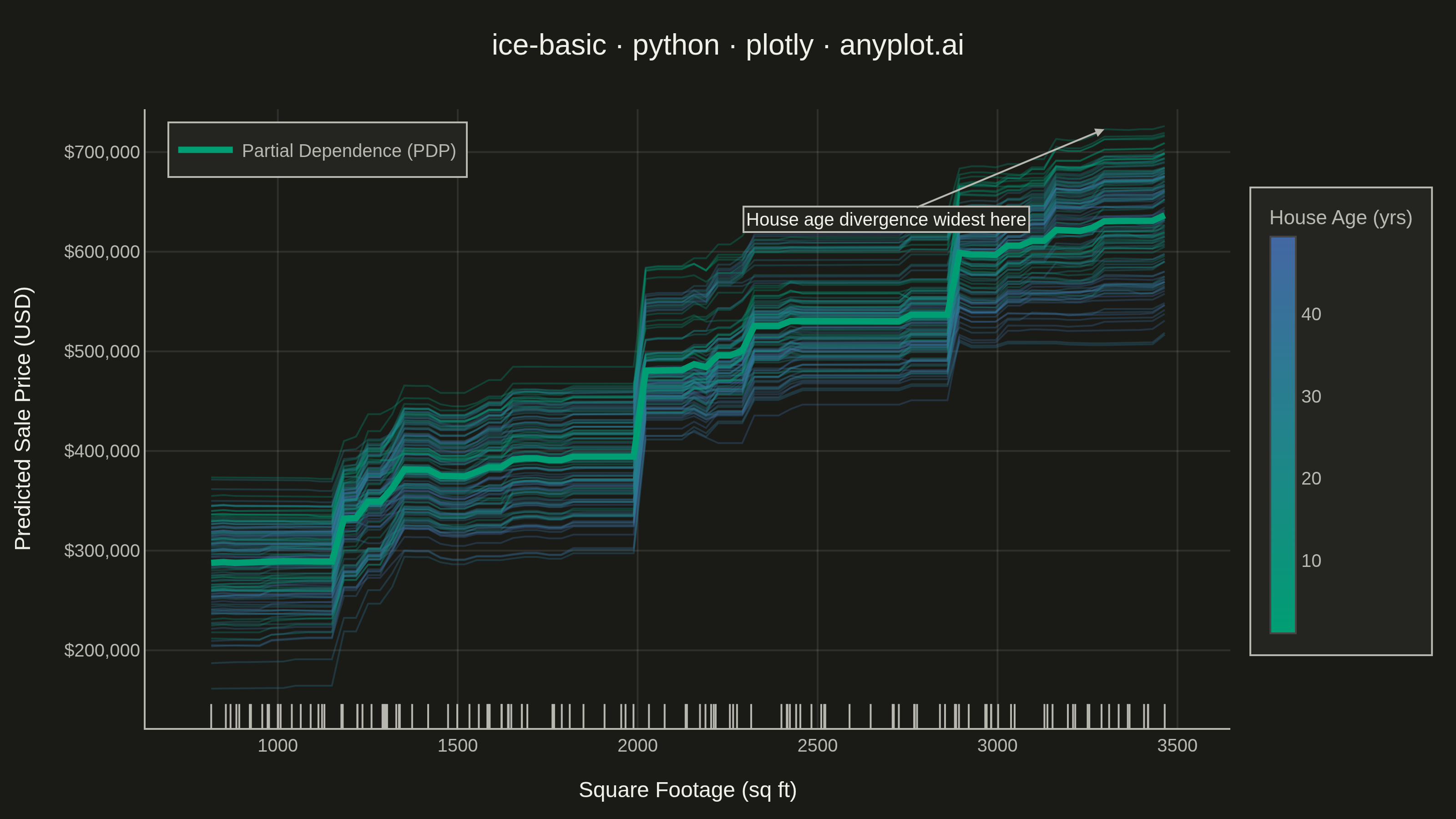
The same plot in 14 other libraries — Python: Altair, Bokeh, lets-plot, Matplotlib, plotnine, Pygal, Seaborn; R: ggplot2; Julia: Makie.jl; JavaScript: Chart.js, D3.js, Apache ECharts, Highcharts, MUI X Charts. Compare all 15 side by side: Individual Conditional Expectation (ICE) Plot in Python, R, Julia and JavaScript.
An Individual Conditional Expectation (ICE) plot visualizes how the predicted outcome of a machine learning model changes for each individual observation as a single feature varies across its range. Unlike partial dependence plots (PDP) that show the average marginal effect, ICE plots display one line per observation, revealing heterogeneous effects, feature interactions, and subgroup-specific behaviors that would be hidden by averaging. This makes ICE plots essential for detecting when a feature's effect varies across the population.
""" anyplot.ai
ice-basic: Individual Conditional Expectation (ICE) Plot
Library: plotly 6.9.0 | Python 3.13.15
Quality: 90/100 | Updated: 2026-08-17
"""

import os
import sys


# Prevent this file (plotly.py) from shadowing the plotly package
_here = os.path.dirname(os.path.abspath(__file__))
sys.path = [p for p in sys.path if os.path.normpath(os.path.abspath(p or ".")) != _here]

import numpy as np
import plotly.colors as pc
import plotly.graph_objects as go
from sklearn.ensemble import GradientBoostingRegressor


# Theme tokens
THEME = os.getenv("ANYPLOT_THEME", "light")
PAGE_BG = "#FAF8F1" if THEME == "light" else "#1A1A17"
ELEVATED_BG = "#FFFDF6" if THEME == "light" else "#242420"
INK = "#1A1A17" if THEME == "light" else "#F0EFE8"
INK_SOFT = "#4A4A44" if THEME == "light" else "#B8B7B0"
GRID = "rgba(26,26,23,0.10)" if THEME == "light" else "rgba(240,239,232,0.10)"
BRAND = "#009E73"

# Data — synthetic housing dataset
np.random.seed(42)
n_houses = 120

sqft = np.random.uniform(800, 3500, n_houses)
bedrooms = np.random.randint(2, 6, n_houses).astype(float)
house_age = np.random.uniform(1, 50, n_houses)
lot_size = np.random.uniform(3000, 15000, n_houses)
neighborhood_score = np.random.uniform(3, 10, n_houses)

sale_price = (
    150 * sqft
    + 8000 * bedrooms
    - 1200 * house_age
    + 5 * lot_size
    + 15000 * neighborhood_score
    + np.random.normal(0, 25000, n_houses)
)

X = np.column_stack([sqft, bedrooms, house_age, lot_size, neighborhood_score])
model = GradientBoostingRegressor(n_estimators=100, max_depth=4, random_state=42)
model.fit(X, sale_price)

# ICE predictions: vary square footage, hold all other features fixed per house
sqft_grid = np.linspace(sqft.min(), sqft.max(), 80)
ice_preds = np.zeros((n_houses, len(sqft_grid)))
for j, val in enumerate(sqft_grid):
    X_mod = X.copy()
    X_mod[:, 0] = val
    ice_preds[:, j] = model.predict(X_mod)

pdp = ice_preds.mean(axis=0)

# ICE line colors from the Imprint sequential colormap, mapped to house age
IMPRINT_SEQ = ["#009E73", "#4467A3"]
age_norm = (house_age - house_age.min()) / (house_age.max() - house_age.min())
raw_colors = pc.sample_colorscale(IMPRINT_SEQ, age_norm.tolist())
ice_colors = [c.replace("rgb(", "rgba(").replace(")", ", 0.30)") for c in raw_colors]

# Plot
fig = go.Figure()

# ICE lines colored by house age (Imprint sequential)
for i in range(n_houses):
    fig.add_trace(
        go.Scatter(
            x=sqft_grid,
            y=ice_preds[i],
            mode="lines",
            line=dict(width=1, color=ice_colors[i]),
            showlegend=False,
            hoverinfo="skip",
        )
    )

# PDP overlay — bold brand-green curve
fig.add_trace(
    go.Scatter(
        x=sqft_grid,
        y=pdp,
        mode="lines",
        name="Partial Dependence (PDP)",
        line=dict(width=3.5, color=BRAND),
        showlegend=True,
    )
)

# Annotate the region where house-age most strongly separates predictions
spread = ice_preds.max(axis=0) - ice_preds.min(axis=0)
divergence_idx = int(np.argmax(spread))
divergence_x = sqft_grid[divergence_idx]
divergence_y = ice_preds[:, divergence_idx].max()

# Rug plot — distribution of observed square footage values
y_range = ice_preds.max() - ice_preds.min()
y_rug = ice_preds.min() - y_range * 0.05
fig.add_trace(
    go.Scatter(
        x=sqft,
        y=[y_rug] * n_houses,
        mode="markers",
        marker=dict(symbol="line-ns", size=10, color=INK_SOFT, line=dict(width=1, color=INK_SOFT)),
        showlegend=False,
        hoverinfo="skip",
    )
)

# Dummy trace to render the house age colorbar
fig.add_trace(
    go.Scatter(
        x=[None],
        y=[None],
        mode="markers",
        marker=dict(
            colorscale=[[0.0, IMPRINT_SEQ[0]], [1.0, IMPRINT_SEQ[1]]],
            color=[house_age.min(), house_age.max()],
            cmin=house_age.min(),
            cmax=house_age.max(),
            colorbar=dict(
                title=dict(text="House Age (yrs)", font=dict(size=11, color=INK_SOFT)),
                tickfont=dict(size=10, color=INK_SOFT),
                thickness=14,
                len=0.75,
                x=1.02,
                bgcolor=ELEVATED_BG,
                bordercolor=INK_SOFT,
                borderwidth=1,
            ),
            showscale=True,
        ),
        showlegend=False,
        hoverinfo="skip",
    )
)

# Style
fig.update_layout(
    autosize=False,
    paper_bgcolor=PAGE_BG,
    plot_bgcolor=PAGE_BG,
    title=dict(text="ice-basic · python · plotly · anyplot.ai", font=dict(size=16, color=INK), x=0.5, xanchor="center"),
    xaxis=dict(
        title=dict(text="Square Footage (sq ft)", font=dict(size=12, color=INK)),
        tickfont=dict(size=10, color=INK_SOFT),
        gridcolor=GRID,
        linecolor=INK_SOFT,
        zerolinecolor=GRID,
        showgrid=True,
        mirror=False,
    ),
    yaxis=dict(
        title=dict(text="Predicted Sale Price (USD)", font=dict(size=12, color=INK)),
        tickfont=dict(size=10, color=INK_SOFT),
        gridcolor=GRID,
        linecolor=INK_SOFT,
        zerolinecolor=GRID,
        showgrid=True,
        tickformat="$,.0f",
        range=[y_rug - y_range * 0.02, ice_preds.max() + y_range * 0.03],
    ),
    legend=dict(
        bgcolor=ELEVATED_BG,
        bordercolor=INK_SOFT,
        borderwidth=1,
        font=dict(size=10, color=INK_SOFT),
        x=0.02,
        y=0.98,
        xanchor="left",
        yanchor="top",
    ),
    margin=dict(l=70, r=110, t=60, b=50),
)

fig.add_annotation(
    x=divergence_x,
    y=divergence_y,
    text="House age divergence widest here",
    showarrow=True,
    arrowhead=2,
    arrowcolor=INK_SOFT,
    ax=-120,
    ay=50,
    font=dict(size=10, color=INK),
    bgcolor=ELEVATED_BG,
    bordercolor=INK_SOFT,
    borderwidth=1,
)

# Save
fig.write_image(f"plot-{THEME}.png", width=800, height=450, scale=4)
fig.write_html(f"plot-{THEME}.html", include_plotlyjs="cdn")
Runnable source as JSON, for any HTTP client: https://api.anyplot.ai/specs/ice-basic/plotly/code. Any spec id and library id listed in llms-full.txt fit the same URL shape; every URL below is complete and callable.
{
  "spec_id": "ice-basic",
  "language": "python",
  "library": "plotly",
  "page": "https://anyplot.ai/ice-basic/python/plotly",
  "hub": "https://anyplot.ai/ice-basic",
  "code_json": "https://api.anyplot.ai/specs/ice-basic/plotly/code",
  "spec_json": "https://api.anyplot.ai/specs/ice-basic",
  "render_light_png": "https://storage.googleapis.com/anyplot-images/plots/ice-basic/python/plotly/plot-light.png",
  "render_dark_png": "https://storage.googleapis.com/anyplot-images/plots/ice-basic/python/plotly/plot-dark.png",
  "interactive_light_html": "https://storage.googleapis.com/anyplot-images/plots/ice-basic/python/plotly/plot-light.html",
  "interactive_dark_html": "https://storage.googleapis.com/anyplot-images/plots/ice-basic/python/plotly/plot-dark.html",
  "quality_score": 90.0,
  "license": "MIT",
  "guide": "https://anyplot.ai/llms.txt"
}
Part of Individual Conditional Expectation (ICE) Plot on anyplot.ai.