The same plot in 14 other libraries — JavaScript: Chart.js, Apache ECharts, Highcharts, MUI X Charts; Python: Altair, Bokeh, lets-plot, Matplotlib, Plotly, plotnine, Pygal, Seaborn; R: ggplot2; Julia: Makie.jl. Compare all 15 side by side: Bollinger Bands Indicator Chart in Python, R, Julia and JavaScript.
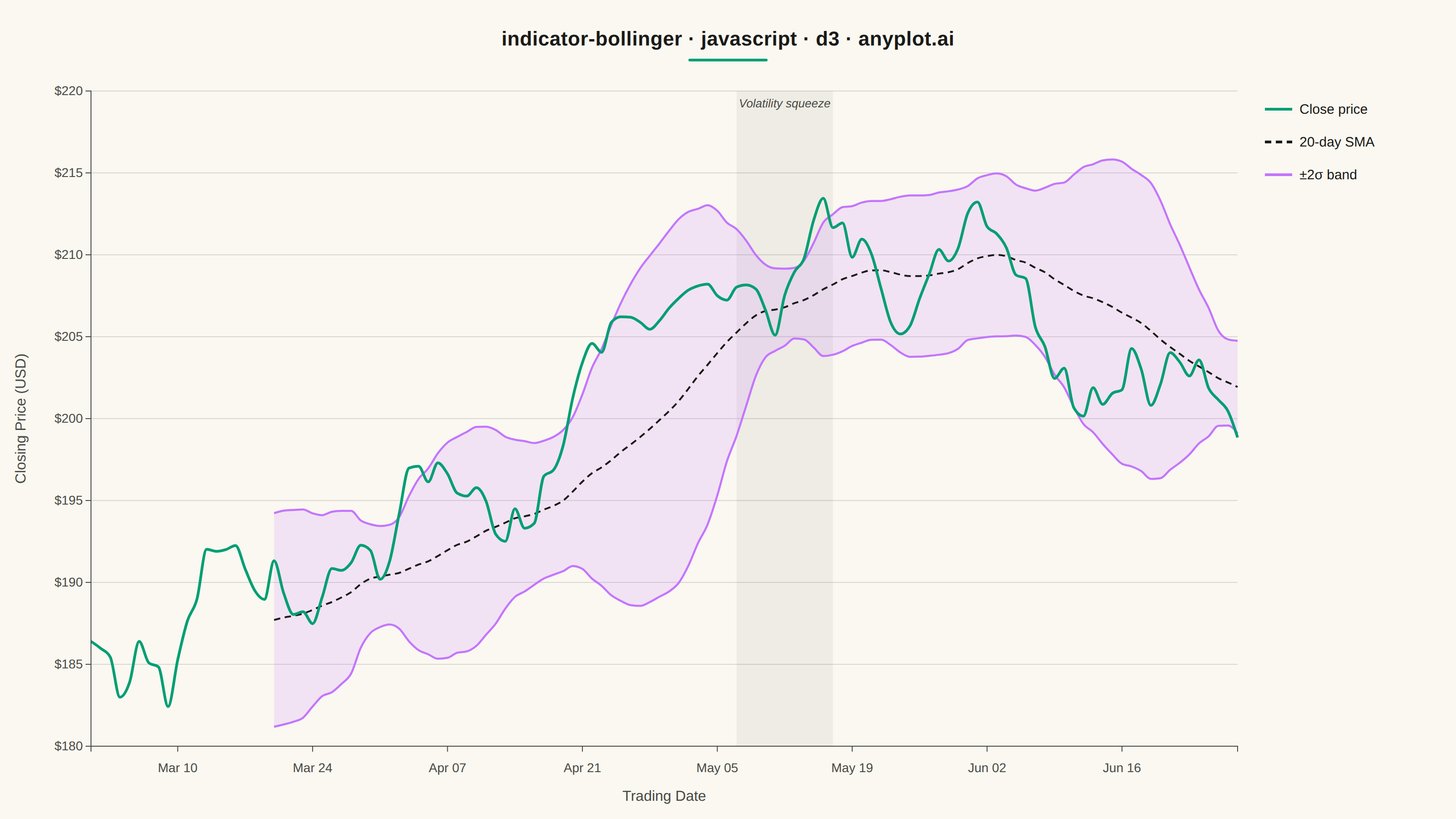
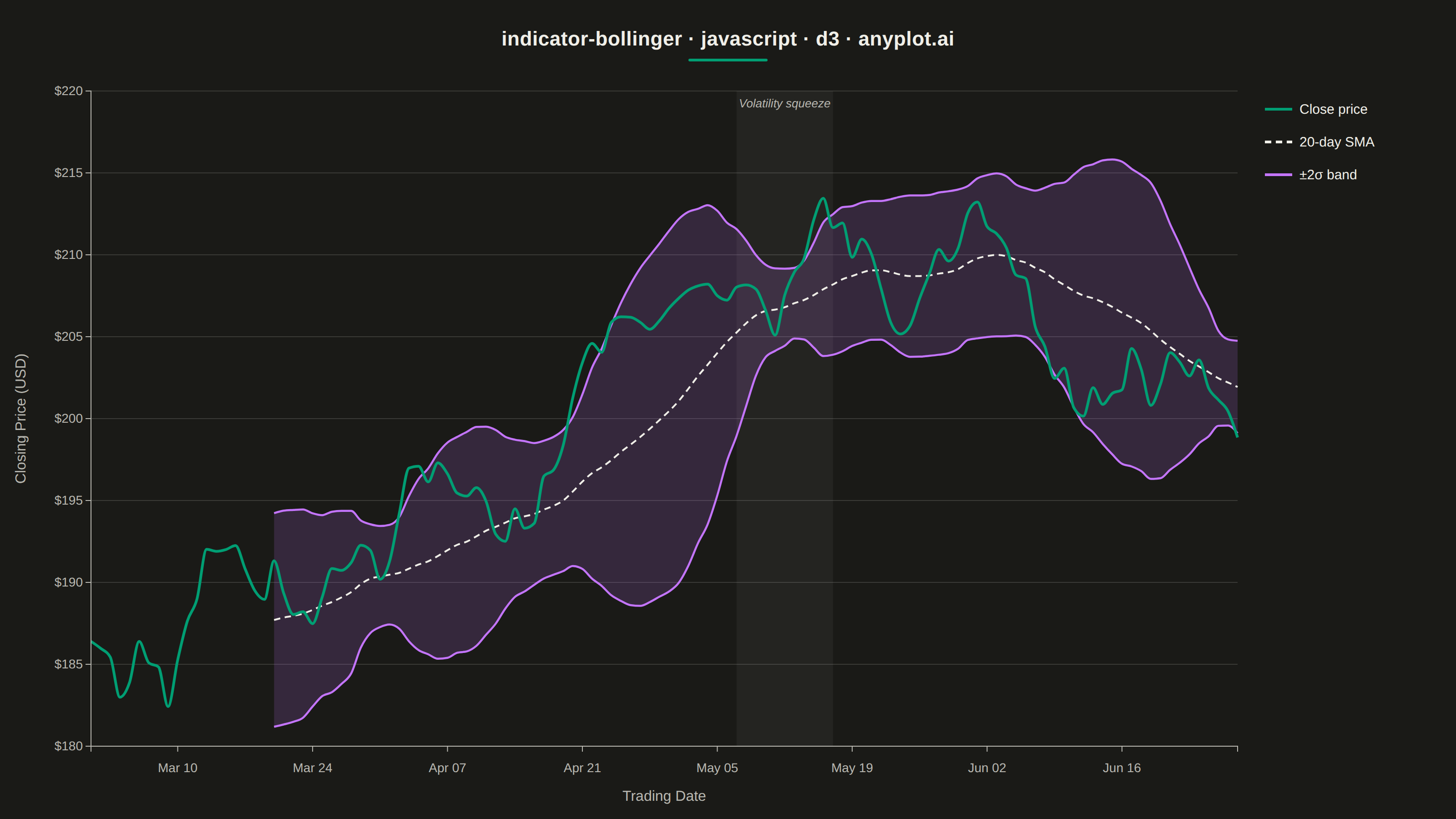
A Bollinger Bands chart displays price data with a volatility envelope consisting of three lines: a middle band (simple moving average), an upper band (SMA plus 2 standard deviations), and a lower band (SMA minus 2 standard deviations). This technical indicator helps traders identify overbought/oversold conditions, volatility patterns, and potential price breakouts by showing how prices relate to their recent statistical range.
// anyplot.ai
// indicator-bollinger: Bollinger Bands Indicator Chart
// Library: d3 7.9.0 | JavaScript 22.23.2
// Quality: 94/100 | Created: 2026-09-02

const t = window.ANYPLOT_TOKENS;
const { width, height } = window.ANYPLOT_SIZE;
const margin = { top: 100, right: 240, bottom: 80, left: 100 };
const iw = width - margin.left - margin.right;
const ih = height - margin.top - margin.bottom;

// --- Data (in-memory, deterministic) ----------------------------------------
// 120 trading days of a synthetic equity close price, generated with a fixed-
// seed LCG random walk. A 20-day SMA + 2 stdev Bollinger envelope is computed
// on top, with a deliberate volatility squeeze mid-series (day 55-70) so the
// band-width contraction/expansion pattern called out in the spec is visible.
let seed = 20260902;
function lcg() {
  seed = (seed * 1664525 + 1013904223) % 4294967296;
  return seed / 4294967296;
}

const WINDOW = 20;
const N = 120;
const startDate = new Date(2024, 2, 1);
const dates = Array.from({ length: N }, (_, i) => {
  const d = new Date(startDate);
  d.setDate(d.getDate() + i);
  return d;
});

const close = [186.4];
for (let i = 1; i < N; i += 1) {
  const squeeze = i >= 55 && i < 70 ? 0.35 : 1; // narrower shocks during the squeeze window
  const drift = 0.12 + 0.35 * Math.sin(i / 22);
  const shock = (lcg() - 0.5) * 5.5 * squeeze;
  close.push(Math.max(60, close[i - 1] + drift + shock));
}

const sma = new Array(N).fill(null);
const upper = new Array(N).fill(null);
const lower = new Array(N).fill(null);
for (let i = WINDOW - 1; i < N; i += 1) {
  const windowSlice = close.slice(i - WINDOW + 1, i + 1);
  const mean = d3.mean(windowSlice);
  const std = d3.deviation(windowSlice);
  sma[i] = mean;
  upper[i] = mean + 2 * std;
  lower[i] = mean - 2 * std;
}

const data = dates.map((date, i) => ({ date, close: close[i], sma: sma[i], upper: upper[i], lower: lower[i] }));
const bandData = data.filter((d) => d.sma !== null);

// --- SVG mount ---------------------------------------------------------------
const svg = d3.select("#container").append("svg").attr("width", width).attr("height", height);
const g = svg.append("g").attr("transform", `translate(${margin.left},${margin.top})`);

// --- Scales --------------------------------------------------------------------
const x = d3.scaleTime().domain(d3.extent(dates)).range([0, iw]);
const y = d3
  .scaleLinear()
  .domain([d3.min(bandData, (d) => d.lower), d3.max(bandData, (d) => d.upper)])
  .nice()
  .range([ih, 0]);

// --- Volatility squeeze annotation (spec-sanctioned callout) -------------------
// The narrowed-shock window (day 55-69) feeds a trailing 20-day rolling stdev,
// so the band itself doesn't visibly pinch until that window is fully inside
// the trailing lookback — around day 67-77. Highlight where the band is
// actually visibly narrow, not where the underlying shocks were dampened.
const squeezeX0 = x(dates[67]);
const squeezeX1 = x(dates[77]);
g.append("rect")
  .attr("x", squeezeX0)
  .attr("y", 0)
  .attr("width", squeezeX1 - squeezeX0)
  .attr("height", ih)
  .attr("fill", t.ink)
  .attr("fill-opacity", 0.05);

g.append("text")
  .attr("x", (squeezeX0 + squeezeX1) / 2)
  .attr("y", 18)
  .attr("text-anchor", "middle")
  .attr("fill", t.inkSoft)
  .style("font-size", "13px")
  .style("font-style", "italic")
  .text("Volatility squeeze");

// --- Gridlines -----------------------------------------------------------------
g.append("g")
  .attr("class", "grid")
  .call(d3.axisLeft(y).tickSize(-iw).tickFormat(""))
  .call((sel) => sel.select(".domain").remove())
  .selectAll("line")
  .attr("stroke", t.grid);

// --- Band fill (semi-transparent, same color for both edges) -------------------
const bandCurve = d3.curveMonotoneX;
const area = d3
  .area()
  .x((d) => x(d.date))
  .y0((d) => y(d.lower))
  .y1((d) => y(d.upper))
  .curve(bandCurve);

g.append("path").datum(bandData).attr("fill", t.palette[1]).attr("fill-opacity", 0.16).attr("d", area);

const upperLine = d3.line().x((d) => x(d.date)).y((d) => y(d.upper)).curve(bandCurve);
g.append("path")
  .datum(bandData)
  .attr("fill", "none")
  .attr("stroke", t.palette[1])
  .attr("stroke-width", 2.25)
  .attr("d", upperLine);

const lowerLine = d3.line().x((d) => x(d.date)).y((d) => y(d.lower)).curve(bandCurve);
g.append("path")
  .datum(bandData)
  .attr("fill", "none")
  .attr("stroke", t.palette[1])
  .attr("stroke-width", 2.25)
  .attr("d", lowerLine);

// --- Middle band (20-day SMA), dashed, ink-neutral reference line --------------
const smaLine = d3.line().x((d) => x(d.date)).y((d) => y(d.sma)).curve(bandCurve);
g.append("path")
  .datum(bandData)
  .attr("fill", "none")
  .attr("stroke", t.ink)
  .attr("stroke-width", 2)
  .attr("stroke-dasharray", "7,5")
  .attr("d", smaLine);

// --- Close price line (brand green, most prominent series) ---------------------
const closeLine = d3
  .line()
  .x((d) => x(d.date))
  .y((d) => y(d.close))
  .curve(d3.curveMonotoneX);

g.append("path").datum(data).attr("fill", "none").attr("stroke", t.palette[0]).attr("stroke-width", 3).attr("d", closeLine);

// --- Axes ------------------------------------------------------------------
const xAxis = g
  .append("g")
  .attr("transform", `translate(0,${ih})`)
  .call(d3.axisBottom(x).ticks(d3.timeWeek.every(2)).tickFormat(d3.timeFormat("%b %d")));
const yAxis = g.append("g").call(d3.axisLeft(y).ticks(6).tickFormat((d) => `$${d}`));

for (const ax of [xAxis, yAxis]) {
  ax.selectAll("text").attr("fill", t.inkSoft).style("font-size", "14px");
  ax.selectAll("line").attr("stroke", t.inkSoft);
  ax.select(".domain").attr("stroke", t.inkSoft);
}
xAxis.selectAll("text").attr("dy", "1.4em");

// --- Axis labels -------------------------------------------------------------
g.append("text")
  .attr("x", iw / 2)
  .attr("y", ih + 60)
  .attr("text-anchor", "middle")
  .attr("fill", t.inkSoft)
  .style("font-size", "16px")
  .text("Trading Date");

g.append("text")
  .attr("transform", "rotate(-90)")
  .attr("x", -ih / 2)
  .attr("y", -72)
  .attr("text-anchor", "middle")
  .attr("fill", t.inkSoft)
  .style("font-size", "16px")
  .text("Closing Price (USD)");

// --- Legend --------------------------------------------------------------------
const legendItems = [
  { label: "Close price", color: t.palette[0], dash: null },
  { label: "20-day SMA", color: t.ink, dash: "7,5" },
  { label: "±2σ band", color: t.palette[1], dash: null },
];

const legend = svg.append("g").attr("transform", `translate(${margin.left + iw + 30}, ${margin.top + 20})`);

const legendRows = legend
  .selectAll("g")
  .data(legendItems)
  .join("g")
  .attr("transform", (_, i) => `translate(0, ${i * 36})`);

legendRows
  .append("line")
  .attr("x1", 0)
  .attr("x2", 30)
  .attr("y1", 0)
  .attr("y2", 0)
  .attr("stroke", (d) => d.color)
  .attr("stroke-width", 3)
  .attr("stroke-dasharray", (d) => d.dash);

legendRows
  .append("text")
  .attr("x", 38)
  .attr("y", 5)
  .attr("fill", t.ink)
  .style("font-size", "15px")
  .text((d) => d.label);

// --- Title ---------------------------------------------------------------------
const title = "indicator-bollinger · javascript · d3 · anyplot.ai";
const titleFontSize = Math.round(22 * Math.min(1, 67 / title.length));
svg
  .append("text")
  .attr("x", width / 2)
  .attr("y", 50)
  .attr("text-anchor", "middle")
  .attr("fill", t.ink)
  .style("font-size", `${titleFontSize}px`)
  .style("font-weight", "600")
  .style("letter-spacing", "0.3px")
  .text(title);

// Brand-green accent rule under the title, echoing the primary close-price series
svg
  .append("line")
  .attr("x1", width / 2 - 42)
  .attr("x2", width / 2 + 42)
  .attr("y1", 66)
  .attr("y2", 66)
  .attr("stroke", t.palette[0])
  .attr("stroke-width", 3)
  .attr("stroke-linecap", "round");
Runnable source as JSON, for any HTTP client: https://api.anyplot.ai/specs/indicator-bollinger/d3/code. Any spec id and library id listed in llms-full.txt fit the same URL shape; every URL below is complete and callable.
{
  "spec_id": "indicator-bollinger",
  "language": "javascript",
  "library": "d3",
  "page": "https://anyplot.ai/indicator-bollinger/javascript/d3",
  "hub": "https://anyplot.ai/indicator-bollinger",
  "code_json": "https://api.anyplot.ai/specs/indicator-bollinger/d3/code",
  "spec_json": "https://api.anyplot.ai/specs/indicator-bollinger",
  "render_light_png": "https://storage.googleapis.com/anyplot-images/plots/indicator-bollinger/javascript/d3/plot-light.png",
  "render_dark_png": "https://storage.googleapis.com/anyplot-images/plots/indicator-bollinger/javascript/d3/plot-dark.png",
  "interactive_light_html": "https://storage.googleapis.com/anyplot-images/plots/indicator-bollinger/javascript/d3/plot-light.html",
  "interactive_dark_html": "https://storage.googleapis.com/anyplot-images/plots/indicator-bollinger/javascript/d3/plot-dark.html",
  "quality_score": 94.0,
  "license": "MIT",
  "guide": "https://anyplot.ai/llms.txt"
}
Part of Bollinger Bands Indicator Chart on anyplot.ai.