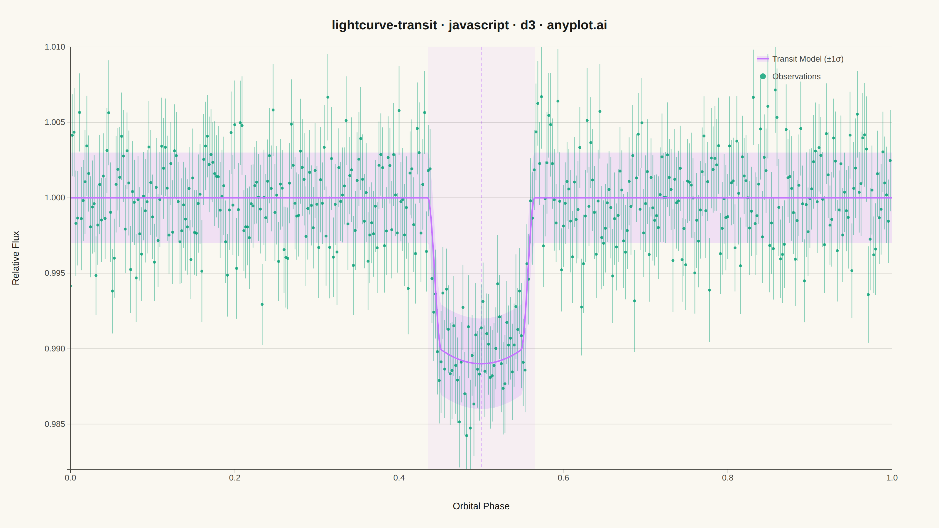
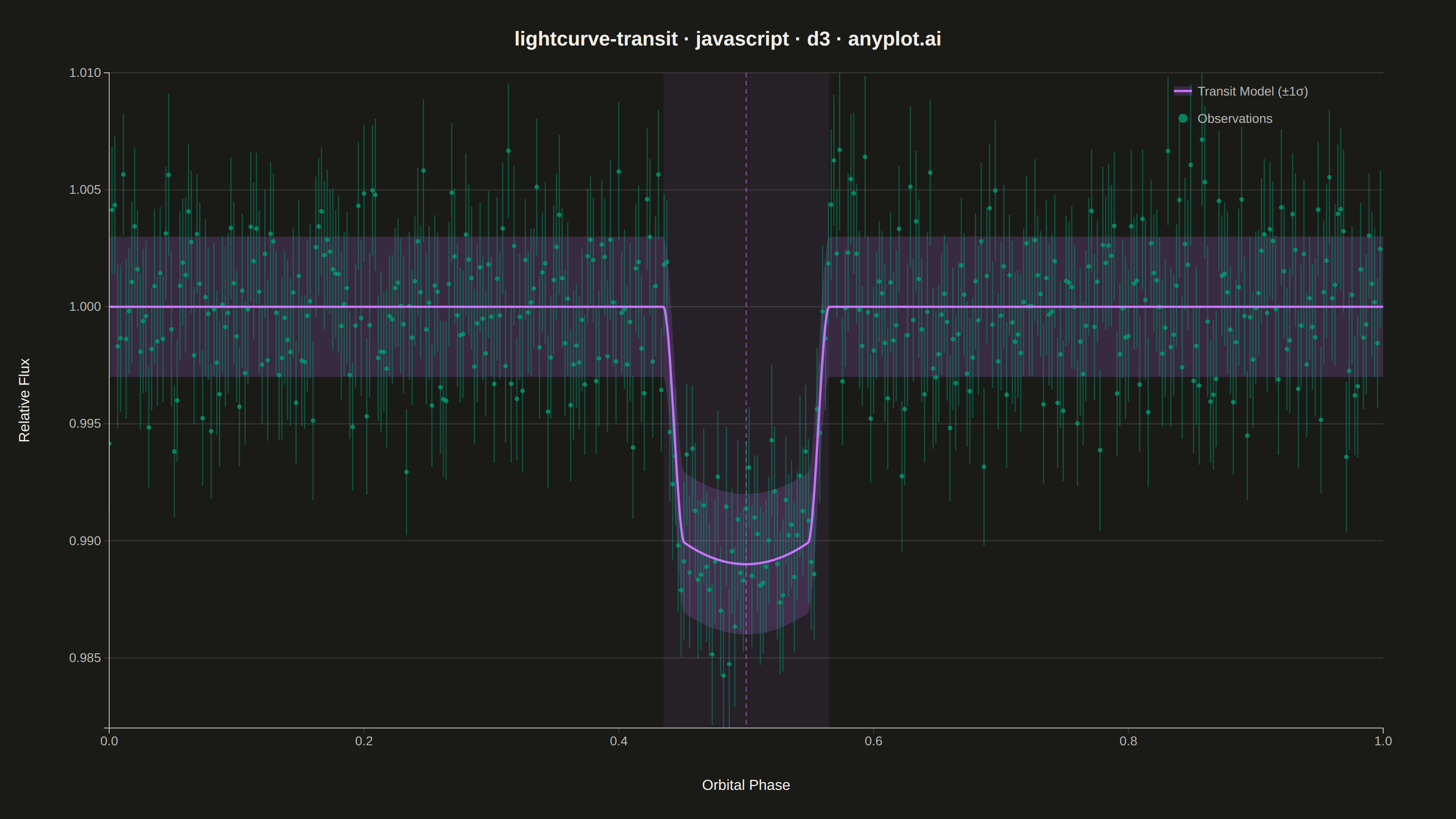
A time-series plot showing the brightness of an astronomical object over time, designed to reveal exoplanet transit events as characteristic dips in flux. The plot displays photometric measurements with error bars against time or orbital phase, with an optional fitted transit model overlay. This visualization is fundamental in observational astronomy for detecting and characterizing planetary transits, variable stars, and other periodic brightness variations.
// anyplot.ai
// lightcurve-transit: Astronomical Light Curve
// Library: d3 7.9.0 | JavaScript 22.22.3
// Quality: 89/100 | Created: 2026-06-20

//# anyplot-orientation: landscape

const t = window.ANYPLOT_TOKENS;
const { width, height } = window.ANYPLOT_SIZE;
const margin = { top: 80, right: 80, bottom: 100, left: 120 };
const iw = width - margin.left - margin.right;
const ih = height - margin.top - margin.bottom;

// Deterministic LCG (seed 42) — browser has no seeded RNG
let _seed = 42;
function lcg() {
  _seed = ((_seed * 1664525) + 1013904223) >>> 0;
  return _seed / 0x100000000;
}
function randn() {
  return Math.sqrt(-2 * Math.log(lcg() + 1e-10)) * Math.cos(2 * Math.PI * lcg());
}

// Transit parameters (shared by model + domain)
const tc = 0.5, halfDur = 0.065, depth = 0.011;

// Transit model: trapezoidal with limb-darkening curvature
function transitFlux(phase) {
  const phi = Math.abs(phase - tc);
  if (phi > halfDur) return 1.0;
  const u = phi / halfDur;
  const depthHere = depth * (1 - 0.15 * u * u);
  const ingressZone = 0.25;
  if (u > 1 - ingressZone) {
    const s = (1 - u) / ingressZone;
    return 1.0 - depthHere * s * s * (3 - 2 * s);
  }
  return 1.0 - depthHere;
}

// Phase-folded observations: 450 points with Gaussian photometric noise
const N = 450;
const obs = Array.from({ length: N }, (_, i) => {
  const phase = i / N;
  const model = transitFlux(phase);
  const fluxErr = 0.0025 + lcg() * 0.0010;
  const flux = model + randn() * 0.0030;
  return { phase, flux, fluxErr };
});

// Smooth model curve with ±1σ band (1001 points for clean rendering)
const sigma1 = 0.003;
const modelCurve = Array.from({ length: 1001 }, (_, i) => {
  const phase = i / 1000;
  const flux = transitFlux(phase);
  return { phase, flux, lo: flux - sigma1, hi: flux + sigma1 };
});

// SVG
const svg = d3.select("#container").append("svg")
  .attr("width", width).attr("height", height);

// Clip-path: keep data elements inside axes bounds — idiomatic D3 pattern
svg.append("defs").append("clipPath")
  .attr("id", "plot-area")
  .append("rect")
  .attr("x", 0).attr("y", 0).attr("width", iw).attr("height", ih);

const g = svg.append("g").attr("transform", `translate(${margin.left},${margin.top})`);

// Scales — tighten Y domain so transit dip fills canvas (avoids 40% empty space)
const transitBase = 1.0 - depth; // ~0.989, the transit floor
const yMin = transitBase - 0.5 * depth; // ~0.9835
const xScale = d3.scaleLinear().domain([0, 1]).range([0, iw]);
const yScale = d3.scaleLinear().domain([yMin, 1.009]).nice().range([ih, 0]);

// Transit window background — visual storytelling: highlight the ingress/egress window
g.append("rect")
  .attr("x", xScale(tc - halfDur))
  .attr("y", 0)
  .attr("width", xScale(tc + halfDur) - xScale(tc - halfDur))
  .attr("height", ih)
  .attr("fill", t.palette[1])
  .attr("opacity", 0.07);

// Dashed vertical at transit midpoint — marks the deepest-flux moment
g.append("line")
  .attr("x1", xScale(tc)).attr("x2", xScale(tc))
  .attr("y1", 0).attr("y2", ih)
  .attr("stroke", t.palette[1])
  .attr("stroke-width", 1.2)
  .attr("stroke-dasharray", "5,4")
  .attr("opacity", 0.6);

// Horizontal grid lines (y-axis only, subtle)
yScale.ticks(6).forEach((tick) => {
  g.append("line")
    .attr("x1", 0).attr("x2", iw)
    .attr("y1", yScale(tick)).attr("y2", yScale(tick))
    .attr("stroke", t.grid).attr("stroke-width", 1);
});

// Clipped group: all data elements stay inside the axes frame
const clipG = g.append("g").attr("clip-path", "url(#plot-area)");

// ±1σ confidence band around model — d3.area() showcases D3's area generator
const bandGen = d3.area()
  .x((d) => xScale(d.phase))
  .y0((d) => yScale(d.lo))
  .y1((d) => yScale(d.hi));

clipG.append("path")
  .datum(modelCurve)
  .attr("fill", t.palette[1])
  .attr("opacity", 0.18)
  .attr("d", bandGen);

// Error bars — drawn below points; stroke-width 1.3 for legibility in transit region
clipG.append("g")
  .selectAll("line")
  .data(obs)
  .join("line")
  .attr("x1", (d) => xScale(d.phase))
  .attr("x2", (d) => xScale(d.phase))
  .attr("y1", (d) => yScale(d.flux - d.fluxErr))
  .attr("y2", (d) => yScale(d.flux + d.fluxErr))
  .attr("stroke", t.palette[0])
  .attr("stroke-width", 1.3)
  .attr("opacity", 0.45);

// Data points — Imprint palette[0] (#009E73) as first series
clipG.append("g")
  .selectAll("circle")
  .data(obs)
  .join("circle")
  .attr("cx", (d) => xScale(d.phase))
  .attr("cy", (d) => yScale(d.flux))
  .attr("r", 2.5)
  .attr("fill", t.palette[0])
  .attr("opacity", 0.80);

// Transit model line — Imprint palette[1] (#C475FD)
const lineGen = d3.line()
  .x((d) => xScale(d.phase))
  .y((d) => yScale(d.flux));
clipG.append("path")
  .datum(modelCurve)
  .attr("fill", "none")
  .attr("stroke", t.palette[1])
  .attr("stroke-width", 2.5)
  .attr("d", lineGen);

// Axes
const xAxis = d3.axisBottom(xScale).ticks(5).tickFormat(d3.format(".1f"));
const yAxis = d3.axisLeft(yScale).ticks(6).tickFormat(d3.format(".3f"));

const gx = g.append("g").attr("transform", `translate(0,${ih})`).call(xAxis);
const gy = g.append("g").call(yAxis);

for (const ax of [gx, gy]) {
  ax.selectAll("text").attr("fill", t.inkSoft).style("font-size", "14px");
  ax.selectAll("line").attr("stroke", t.grid);
  ax.select(".domain").attr("stroke", t.inkSoft);
}

// Axis labels
g.append("text")
  .attr("x", iw / 2).attr("y", ih + 68)
  .attr("text-anchor", "middle")
  .attr("fill", t.ink).style("font-size", "16px")
  .text("Orbital Phase");

g.append("text")
  .attr("transform", "rotate(-90)")
  .attr("x", -(ih / 2)).attr("y", -88)
  .attr("text-anchor", "middle")
  .attr("fill", t.ink).style("font-size", "16px")
  .text("Relative Flux");

// Legend
const lx = iw - 220, ly = 20;

// Transit model: confidence band swatch + line
g.append("rect")
  .attr("x", lx - 10).attr("y", ly - 5)
  .attr("width", 20).attr("height", 10)
  .attr("fill", t.palette[1]).attr("opacity", 0.18);
g.append("line")
  .attr("x1", lx - 10).attr("x2", lx + 10)
  .attr("y1", ly).attr("y2", ly)
  .attr("stroke", t.palette[1]).attr("stroke-width", 2.5);
g.append("text")
  .attr("x", lx + 16).attr("y", ly + 5)
  .attr("fill", t.inkSoft).style("font-size", "14px")
  .text("Transit Model (±1σ)");

// Observations
g.append("circle")
  .attr("cx", lx).attr("cy", ly + 30)
  .attr("r", 5)
  .attr("fill", t.palette[0]).attr("opacity", 0.80);
g.append("text")
  .attr("x", lx + 16).attr("y", ly + 35)
  .attr("fill", t.inkSoft).style("font-size", "14px")
  .text("Observations");

// Title
svg.append("text")
  .attr("x", width / 2).attr("y", 50)
  .attr("text-anchor", "middle")
  .attr("fill", t.ink)
  .style("font-size", "22px").style("font-weight", "600")
  .text("lightcurve-transit · javascript · d3 · anyplot.ai");
Runnable source as JSON, for any HTTP client: https://api.anyplot.ai/specs/lightcurve-transit/d3/code. Any spec id and library id listed in llms-full.txt fit the same URL shape; every URL below is complete and callable.
{
  "spec_id": "lightcurve-transit",
  "language": "javascript",
  "library": "d3",
  "page": "https://anyplot.ai/lightcurve-transit/javascript/d3",
  "hub": "https://anyplot.ai/lightcurve-transit",
  "code_json": "https://api.anyplot.ai/specs/lightcurve-transit/d3/code",
  "spec_json": "https://api.anyplot.ai/specs/lightcurve-transit",
  "render_light_png": "https://storage.googleapis.com/anyplot-images/plots/lightcurve-transit/javascript/d3/plot-light.png",
  "render_dark_png": "https://storage.googleapis.com/anyplot-images/plots/lightcurve-transit/javascript/d3/plot-dark.png",
  "interactive_light_html": "https://storage.googleapis.com/anyplot-images/plots/lightcurve-transit/javascript/d3/plot-light.html",
  "interactive_dark_html": "https://storage.googleapis.com/anyplot-images/plots/lightcurve-transit/javascript/d3/plot-dark.html",
  "quality_score": 89.0,
  "license": "MIT",
  "guide": "https://anyplot.ai/llms.txt"
}
Part of Astronomical Light Curve on anyplot.ai.