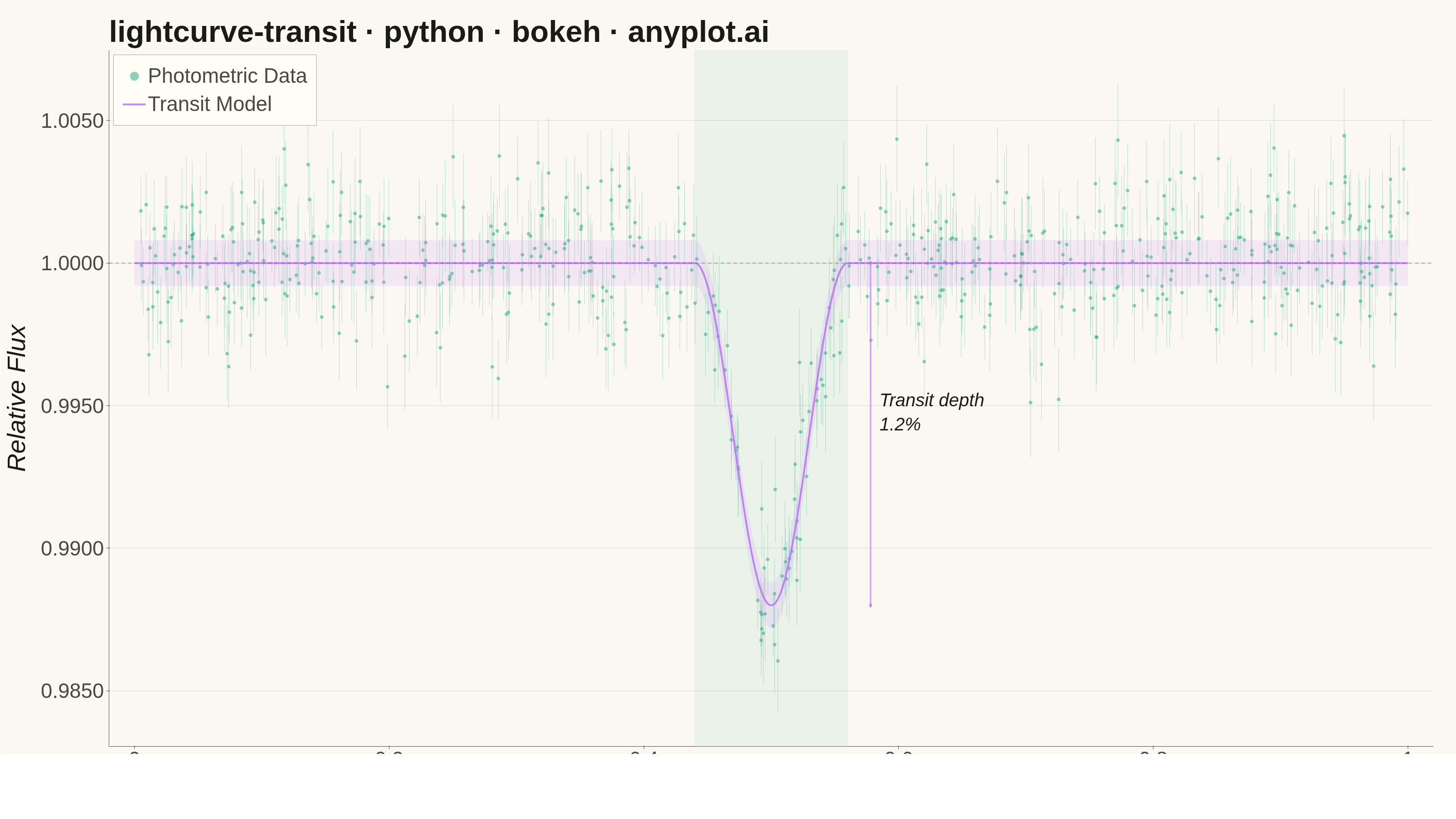
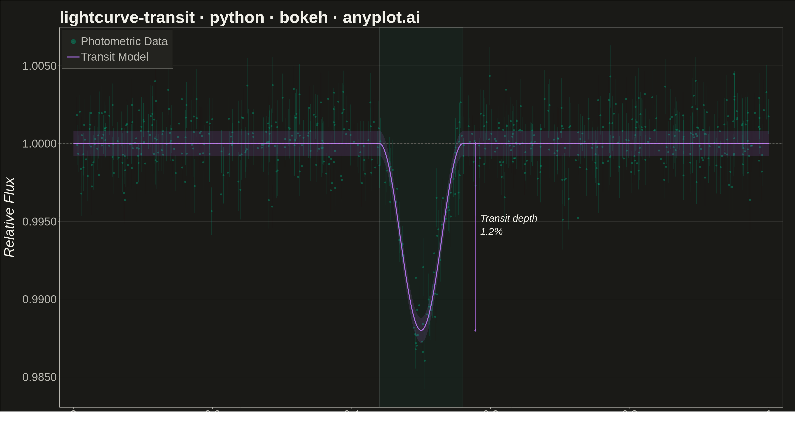
A time-series plot showing the brightness of an astronomical object over time, designed to reveal exoplanet transit events as characteristic dips in flux. The plot displays photometric measurements with error bars against time or orbital phase, with an optional fitted transit model overlay. This visualization is fundamental in observational astronomy for detecting and characterizing planetary transits, variable stars, and other periodic brightness variations.
""" anyplot.ai
lightcurve-transit: Astronomical Light Curve
Library: bokeh 3.9.1 | Python 3.13.14
Quality: 90/100 | Updated: 2026-06-20
"""

import base64
import os
import time
from pathlib import Path

import numpy as np
from bokeh.io import output_file, save
from bokeh.models import (
    Band,
    BoxAnnotation,
    ColumnDataSource,
    CustomJSTickFormatter,
    HoverTool,
    Label,
    Range1d,
    Span,
    Whisker,
)
from bokeh.plotting import figure
from selenium import webdriver
from selenium.webdriver.chrome.options import Options


# Theme tokens — Imprint palette chrome
THEME = os.getenv("ANYPLOT_THEME", "light")
PAGE_BG = "#FAF8F1" if THEME == "light" else "#1A1A17"
ELEVATED_BG = "#FFFDF6" if THEME == "light" else "#242420"
INK = "#1A1A17" if THEME == "light" else "#F0EFE8"
INK_SOFT = "#4A4A44" if THEME == "light" else "#B8B7B0"
INK_MUTED = "#6B6A63" if THEME == "light" else "#A8A79F"

# Imprint categorical palette — canonical order, theme-independent
BRAND = "#009E73"  # position 1 — always first series (photometric data)
MODEL_COLOR = "#C475FD"  # position 2 — transit model curve

# Data — simulated phase-folded exoplanet transit (hot Jupiter style)
np.random.seed(42)
n_points = 600
phase = np.sort(np.random.uniform(0.0, 1.0, n_points))

transit_center = 0.5
transit_depth = 0.012  # ~1.2% flux dip
half_duration = 0.06

dist = np.abs(phase - transit_center)
in_transit = dist < half_duration
model_flux = np.ones(n_points)
model_flux[in_transit] = 1.0 - transit_depth * (0.5 + 0.5 * np.cos(np.pi * dist[in_transit] / half_duration))

flux_err = np.random.uniform(0.001, 0.002, n_points)
flux = model_flux + np.random.normal(0, 1, n_points) * flux_err

# Smooth model curve for the overlay
phase_model = np.linspace(0.0, 1.0, 3000)
dist_m = np.abs(phase_model - transit_center)
in_transit_m = dist_m < half_duration
model_smooth = np.ones(3000)
model_smooth[in_transit_m] = 1.0 - transit_depth * (0.5 + 0.5 * np.cos(np.pi * dist_m[in_transit_m] / half_duration))

source_data = ColumnDataSource(
    data={"phase": phase, "flux": flux, "flux_err": flux_err, "upper": flux + flux_err, "lower": flux - flux_err}
)
source_model = ColumnDataSource(
    data={"phase": phase_model, "model": model_smooth, "upper": model_smooth + 0.0008, "lower": model_smooth - 0.0008}
)

y_min = min(flux.min(), model_smooth.min()) - 0.003
y_max = max(flux.max(), model_smooth.max()) + 0.003

# Plot
title = "lightcurve-transit · python · bokeh · anyplot.ai"

p = figure(
    width=3200,
    height=1800,
    title=title,
    x_axis_label="Orbital Phase",
    y_axis_label="Relative Flux",
    x_range=Range1d(-0.02, 1.02),
    y_range=Range1d(y_min, y_max),
    toolbar_location=None,
    min_border_bottom=160,
    min_border_left=180,
    min_border_top=110,
    min_border_right=50,
)

# Theme chrome
p.background_fill_color = PAGE_BG
p.border_fill_color = PAGE_BG
p.outline_line_color = None

# Transit window highlight (subtle shaded box)
transit_box = BoxAnnotation(
    left=transit_center - half_duration, right=transit_center + half_duration, fill_color=BRAND, fill_alpha=0.06
)
p.add_layout(transit_box)

# Baseline reference at flux = 1.0
baseline = Span(location=1.0, dimension="width", line_color=INK_SOFT, line_width=2, line_dash=[8, 6], line_alpha=0.4)
p.add_layout(baseline)

# Confidence band around transit model
band = Band(
    base="phase",
    upper="upper",
    lower="lower",
    source=source_model,
    fill_color=MODEL_COLOR,
    fill_alpha=0.12,
    line_color=None,
)
p.add_layout(band)

# Error bars — increased alpha for visibility
whisker = Whisker(
    base="phase", upper="upper", lower="lower", source=source_data, line_color=BRAND, line_alpha=0.3, line_width=1
)
whisker.upper_head.size = 0
whisker.lower_head.size = 0
p.add_layout(whisker)

# Data scatter — photometric measurements
scatter_r = p.scatter(
    x="phase",
    y="flux",
    source=source_data,
    size=8,
    color=BRAND,
    alpha=0.45,
    line_color=PAGE_BG,
    line_width=0.5,
    legend_label="Photometric Data",
)

# Transit model curve
p.line(
    x="phase",
    y="model",
    source=source_model,
    line_color=MODEL_COLOR,
    line_width=4,
    line_alpha=0.9,
    legend_label="Transit Model",
)

# Transit depth annotation — vertical line + label quantifying the dip
p.line(
    x=[transit_center + half_duration + 0.018] * 2,
    y=[1.0, 1.0 - transit_depth],
    line_color=MODEL_COLOR,
    line_width=3,
    line_alpha=0.7,
)
p.scatter(
    x=[transit_center + half_duration + 0.018] * 2,
    y=[1.0, 1.0 - transit_depth],
    size=10,
    color=MODEL_COLOR,
    marker="diamond",
    alpha=0.8,
)
depth_label = Label(
    x=transit_center + half_duration + 0.025,
    y=1.0 - transit_depth / 2,
    text=f"Transit depth\n{transit_depth * 100:.1f}%",
    text_font_size="30pt",
    text_color=INK,
    text_font_style="italic",
    text_align="left",
)
p.add_layout(depth_label)

# HoverTool for interactive exploration
hover = HoverTool(
    renderers=[scatter_r],
    tooltips=[("Phase", "@phase{0.0000}"), ("Flux", "@flux{0.00000}"), ("Error", "±@flux_err{0.00000}")],
    mode="mouse",
)
p.add_tools(hover)

# 4-decimal y-axis formatter for scientific precision
p.yaxis.formatter = CustomJSTickFormatter(code="return tick.toFixed(4);")

# Typography — standard 3200×1800 sizes
p.title.text_font_size = "50pt"
p.title.text_color = INK
p.title.text_font_style = "bold"
p.xaxis.axis_label_text_font_size = "42pt"
p.yaxis.axis_label_text_font_size = "42pt"
p.xaxis.axis_label_text_color = INK
p.yaxis.axis_label_text_color = INK
p.xaxis.axis_label_standoff = 20
p.yaxis.axis_label_standoff = 20
p.xaxis.major_label_text_font_size = "34pt"
p.yaxis.major_label_text_font_size = "34pt"
p.xaxis.major_label_text_color = INK_SOFT
p.yaxis.major_label_text_color = INK_SOFT

# Axis lines and ticks
p.xaxis.axis_line_color = INK_SOFT
p.yaxis.axis_line_color = INK_SOFT
p.xaxis.major_tick_line_color = INK_SOFT
p.yaxis.major_tick_line_color = INK_SOFT
p.xaxis.minor_tick_line_color = None
p.yaxis.minor_tick_line_color = None

# Grid — y-axis only, very subtle
p.xgrid.grid_line_color = None
p.ygrid.grid_line_color = INK
p.ygrid.grid_line_alpha = 0.15

# Legend
p.legend.location = "top_left"
p.legend.label_text_font_size = "34pt"
p.legend.label_text_color = INK_SOFT
p.legend.background_fill_color = ELEVATED_BG
p.legend.border_line_color = INK_SOFT
p.legend.padding = 20
p.legend.spacing = 10
p.legend.glyph_height = 50
p.legend.glyph_width = 50

# Save HTML
output_file(f"plot-{THEME}.html")
save(p)

# Screenshot with headless Chrome (Selenium — export_png is not available in CI)
W, H = 3200, 1800
opts = Options()
for arg in (
    "--headless=new",
    "--no-sandbox",
    "--disable-dev-shm-usage",
    "--disable-gpu",
    f"--window-size={W},{H}",
    "--hide-scrollbars",
):
    opts.add_argument(arg)
driver = webdriver.Chrome(options=opts)
driver.set_window_size(W, H)
driver.get(f"file://{Path(f'plot-{THEME}.html').resolve()}")
time.sleep(3)
# CDP screenshot at exact canvas dimensions — avoids viewport-height caps in headless Chrome
result = driver.execute_cdp_cmd(
    "Page.captureScreenshot", {"format": "png", "clip": {"x": 0, "y": 0, "width": W, "height": H, "scale": 1}}
)
with open(f"plot-{THEME}.png", "wb") as fh:
    fh.write(base64.b64decode(result["data"]))
driver.quit()
Runnable source as JSON, for any HTTP client: https://api.anyplot.ai/specs/lightcurve-transit/bokeh/code. Any spec id and library id listed in llms-full.txt fit the same URL shape; every URL below is complete and callable.
{
  "spec_id": "lightcurve-transit",
  "language": "python",
  "library": "bokeh",
  "page": "https://anyplot.ai/lightcurve-transit/python/bokeh",
  "hub": "https://anyplot.ai/lightcurve-transit",
  "code_json": "https://api.anyplot.ai/specs/lightcurve-transit/bokeh/code",
  "spec_json": "https://api.anyplot.ai/specs/lightcurve-transit",
  "render_light_png": "https://storage.googleapis.com/anyplot-images/plots/lightcurve-transit/python/bokeh/plot-light.png",
  "render_dark_png": "https://storage.googleapis.com/anyplot-images/plots/lightcurve-transit/python/bokeh/plot-dark.png",
  "interactive_light_html": "https://storage.googleapis.com/anyplot-images/plots/lightcurve-transit/python/bokeh/plot-light.html",
  "interactive_dark_html": "https://storage.googleapis.com/anyplot-images/plots/lightcurve-transit/python/bokeh/plot-dark.html",
  "quality_score": 90.0,
  "license": "MIT",
  "guide": "https://anyplot.ai/llms.txt"
}
Part of Astronomical Light Curve on anyplot.ai.