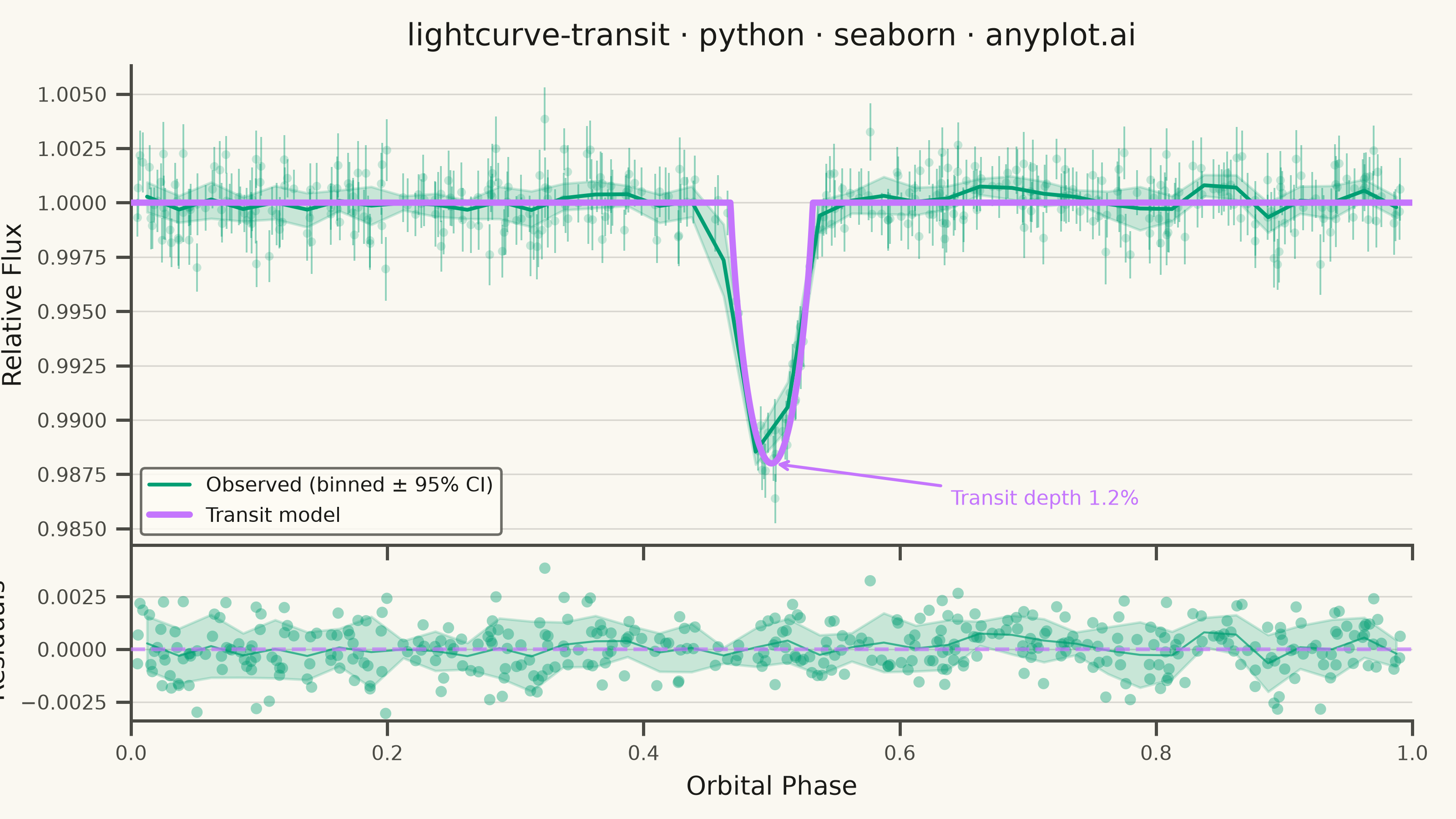
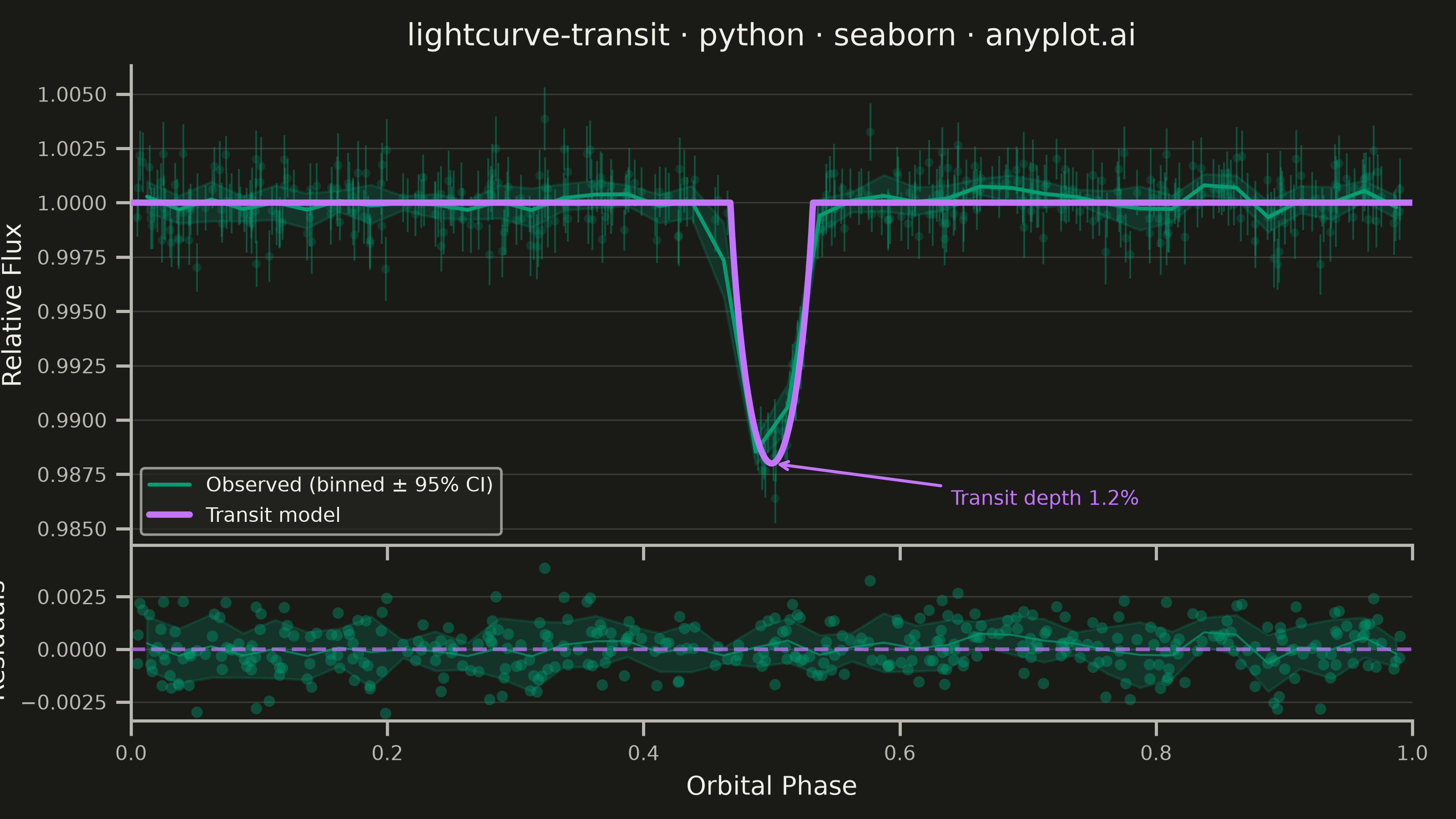
A time-series plot showing the brightness of an astronomical object over time, designed to reveal exoplanet transit events as characteristic dips in flux. The plot displays photometric measurements with error bars against time or orbital phase, with an optional fitted transit model overlay. This visualization is fundamental in observational astronomy for detecting and characterizing planetary transits, variable stars, and other periodic brightness variations.
""" anyplot.ai
lightcurve-transit: Astronomical Light Curve
Library: seaborn 0.13.2 | Python 3.13.14
Quality: 87/100 | Updated: 2026-06-20
"""

import os

import matplotlib.pyplot as plt
import numpy as np
import pandas as pd
import seaborn as sns


# Theme tokens — Imprint palette, theme-adaptive chrome
THEME = os.getenv("ANYPLOT_THEME", "light")
PAGE_BG = "#FAF8F1" if THEME == "light" else "#1A1A17"
ELEVATED_BG = "#FFFDF6" if THEME == "light" else "#242420"
INK = "#1A1A17" if THEME == "light" else "#F0EFE8"
INK_SOFT = "#4A4A44" if THEME == "light" else "#B8B7B0"

# Imprint palette — canonical order, position 1 always first series
DATA_COLOR = "#009E73"  # position 1, brand green — observed flux
MODEL_COLOR = "#C475FD"  # position 2, lavender — transit model

sns.set_theme(
    style="ticks",
    rc={
        "figure.facecolor": PAGE_BG,
        "axes.facecolor": PAGE_BG,
        "axes.edgecolor": INK_SOFT,
        "axes.labelcolor": INK,
        "text.color": INK,
        "xtick.color": INK_SOFT,
        "ytick.color": INK_SOFT,
        "grid.color": INK,
        "grid.alpha": 0.15,
        "legend.facecolor": ELEVATED_BG,
        "legend.edgecolor": INK_SOFT,
    },
)

# Data — wider transit (0.032), 400 pts, u1=0.5/u2=0.3 limb darkening for visual independence
np.random.seed(42)

n_points = 400
phase = np.sort(np.random.uniform(0.0, 1.0, n_points))

transit_center = 0.5
transit_width = 0.032
transit_depth = 0.012
u1, u2 = 0.5, 0.3

z = np.abs(phase - transit_center) / transit_width
dip = np.where(z < 1.0, np.sqrt(np.clip(1.0 - z**2, 0, None)), 0.0)
limb = 1.0 - u1 * (1 - dip) - u2 * (1 - dip) ** 2
model_flux = 1.0 - transit_depth * dip * limb

flux_err = np.random.uniform(0.0008, 0.0015, n_points)
flux = model_flux + np.random.normal(0, 1, n_points) * flux_err
residuals = flux - model_flux

phase_model = np.linspace(0.0, 1.0, 2000)
z_model = np.abs(phase_model - transit_center) / transit_width
dip_model = np.where(z_model < 1.0, np.sqrt(np.clip(1.0 - z_model**2, 0, None)), 0.0)
limb_model = 1.0 - u1 * (1 - dip_model) - u2 * (1 - dip_model) ** 2
model_smooth = 1.0 - transit_depth * dip_model * limb_model

# Phase binning — 40 bins × ~10 pts each for seaborn statistical aggregation
n_bins = 40
phase_edges = np.linspace(0.0, 1.0, n_bins + 1)
phase_centers = 0.5 * (phase_edges[:-1] + phase_edges[1:])
bin_idx = np.clip(np.digitize(phase, phase_edges) - 1, 0, n_bins - 1)

df = pd.DataFrame(
    {"phase": phase, "phase_bin": phase_centers[bin_idx], "flux": flux, "flux_err": flux_err, "residuals": residuals}
)
df_model = pd.DataFrame({"phase": phase_model, "flux": model_smooth})

# Plot — landscape canvas: figsize=(8, 4.5) × dpi=400 → 3200×1800 px
fig, (ax_main, ax_resid) = plt.subplots(
    2, 1, figsize=(8, 4.5), dpi=400, height_ratios=[3, 1], sharex=True, gridspec_kw={"hspace": 0.05}, facecolor=PAGE_BG
)

# Main panel: error bars (visible precision layer behind scatter)
ax_main.errorbar(
    df["phase"],
    df["flux"],
    yerr=df["flux_err"],
    fmt="none",
    ecolor=DATA_COLOR,
    elinewidth=0.7,
    alpha=0.42,
    capsize=0,
    zorder=1,
)

# Main panel: individual scatter (faint texture showing raw data density)
sns.scatterplot(
    data=df,
    x="phase",
    y="flux",
    color=DATA_COLOR,
    s=12,
    alpha=0.22,
    edgecolor="none",
    ax=ax_main,
    zorder=2,
    legend=False,
)

# Main panel: phase-binned mean with 95% CI band — seaborn statistical aggregation
sns.lineplot(
    data=df,
    x="phase_bin",
    y="flux",
    color=DATA_COLOR,
    estimator="mean",
    errorbar=("ci", 95),
    linewidth=1.5,
    ax=ax_main,
    zorder=3,
    label="Observed (binned ± 95% CI)",
)

# Main panel: transit model curve
sns.lineplot(
    data=df_model, x="phase", y="flux", color=MODEL_COLOR, linewidth=2.5, ax=ax_main, zorder=4, label="Transit model"
)

# Residuals panel: scatter points
sns.scatterplot(
    data=df, x="phase", y="residuals", color=DATA_COLOR, s=20, alpha=0.40, edgecolor="none", ax=ax_resid, legend=False
)

# Residuals panel: phase-binned mean ± SD band — shows absence of systematic residual structure
sns.lineplot(
    data=df,
    x="phase_bin",
    y="residuals",
    color=DATA_COLOR,
    estimator="mean",
    errorbar="sd",
    linewidth=0.8,
    alpha=0.70,
    ax=ax_resid,
    legend=False,
)
ax_resid.axhline(0, color=MODEL_COLOR, linewidth=1.5, linestyle="--", alpha=0.7, zorder=3)

# Transit depth annotation — highlights key scientific measurement
transit_min = model_smooth.min()
ax_main.annotate(
    f"Transit depth {transit_depth * 100:.1f}%",
    xy=(transit_center, transit_min),
    xytext=(transit_center + 0.14, transit_min - 0.0012),
    fontsize=8,
    color=MODEL_COLOR,
    fontweight="medium",
    arrowprops={"arrowstyle": "->", "color": MODEL_COLOR, "lw": 1.2},
    ha="left",
    va="top",
    zorder=5,
)

# Style — main panel
ax_main.set_facecolor(PAGE_BG)
ax_main.set_ylabel("Relative Flux", fontsize=10, color=INK)
ax_main.set_title(
    "lightcurve-transit · python · seaborn · anyplot.ai", fontsize=12, fontweight="medium", color=INK, pad=8
)
ax_main.tick_params(axis="both", labelsize=8, colors=INK_SOFT)
ax_main.tick_params(axis="x", labelbottom=False)
ax_main.yaxis.grid(True, alpha=0.15, linewidth=0.6, color=INK)
ax_main.legend(fontsize=8, frameon=True, loc="lower left")

# Style — residuals panel
ax_resid.set_facecolor(PAGE_BG)
ax_resid.set_xlabel("Orbital Phase", fontsize=10, color=INK)
ax_resid.set_ylabel("Residuals", fontsize=10, color=INK)
ax_resid.tick_params(axis="both", labelsize=8, colors=INK_SOFT)
ax_resid.yaxis.grid(True, alpha=0.15, linewidth=0.6, color=INK)
ax_resid.set_xlim(0.0, 1.0)

# Despine both panels
sns.despine(ax=ax_main)
sns.despine(ax=ax_resid)

fig.subplots_adjust(left=0.09, right=0.97, top=0.92, bottom=0.12)

# Save — no bbox_inches='tight' (seaborn canvas contract: figsize × dpi = exact pixel target)
plt.savefig(f"plot-{THEME}.png", dpi=400, facecolor=PAGE_BG)
Runnable source as JSON, for any HTTP client: https://api.anyplot.ai/specs/lightcurve-transit/seaborn/code. Any spec id and library id listed in llms-full.txt fit the same URL shape; every URL below is complete and callable.
{
  "spec_id": "lightcurve-transit",
  "language": "python",
  "library": "seaborn",
  "page": "https://anyplot.ai/lightcurve-transit/python/seaborn",
  "hub": "https://anyplot.ai/lightcurve-transit",
  "code_json": "https://api.anyplot.ai/specs/lightcurve-transit/seaborn/code",
  "spec_json": "https://api.anyplot.ai/specs/lightcurve-transit",
  "render_light_png": "https://storage.googleapis.com/anyplot-images/plots/lightcurve-transit/python/seaborn/plot-light.png",
  "render_dark_png": "https://storage.googleapis.com/anyplot-images/plots/lightcurve-transit/python/seaborn/plot-dark.png",
  "quality_score": 87.0,
  "license": "MIT",
  "guide": "https://anyplot.ai/llms.txt"
}
Part of Astronomical Light Curve on anyplot.ai.