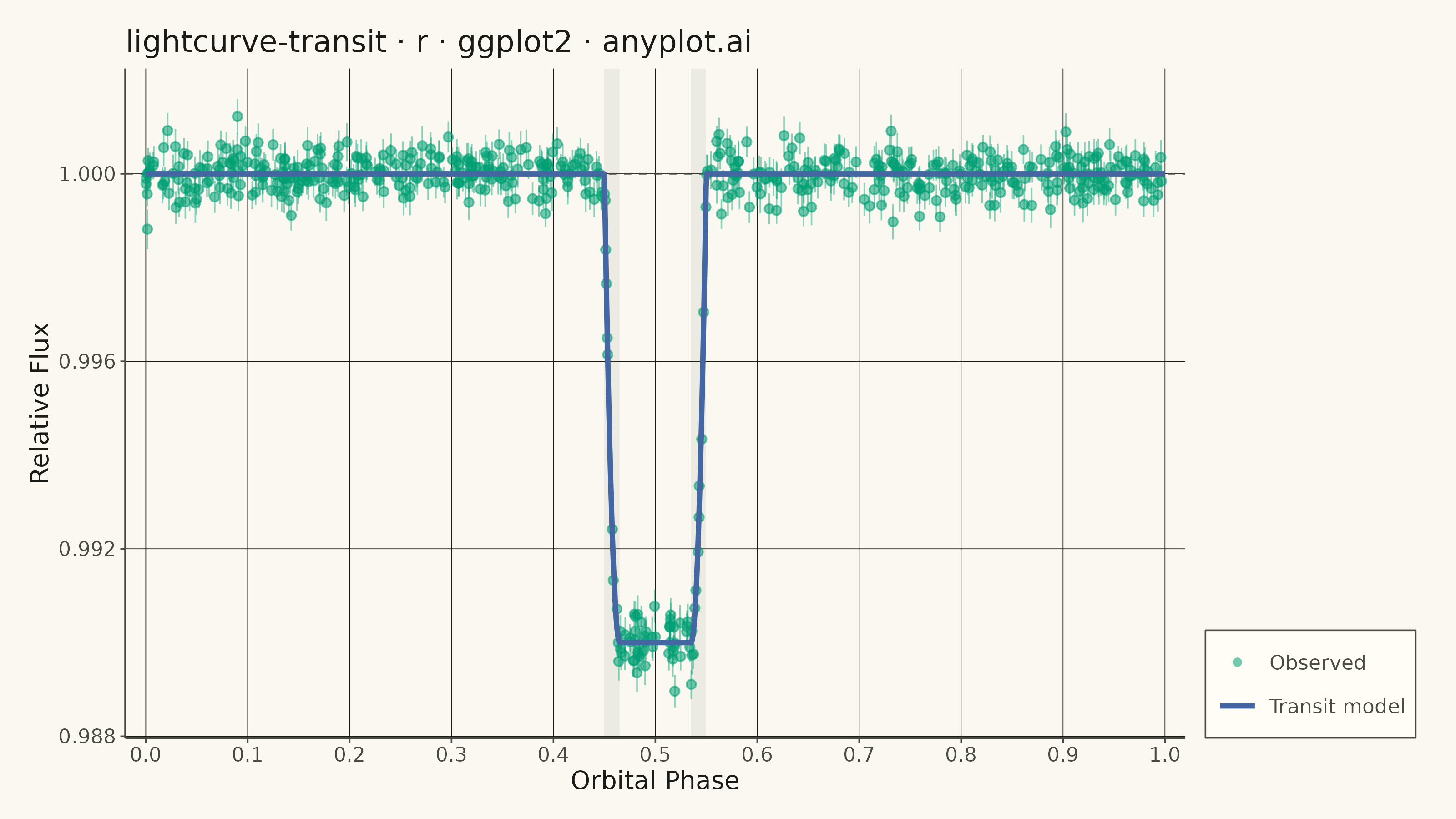
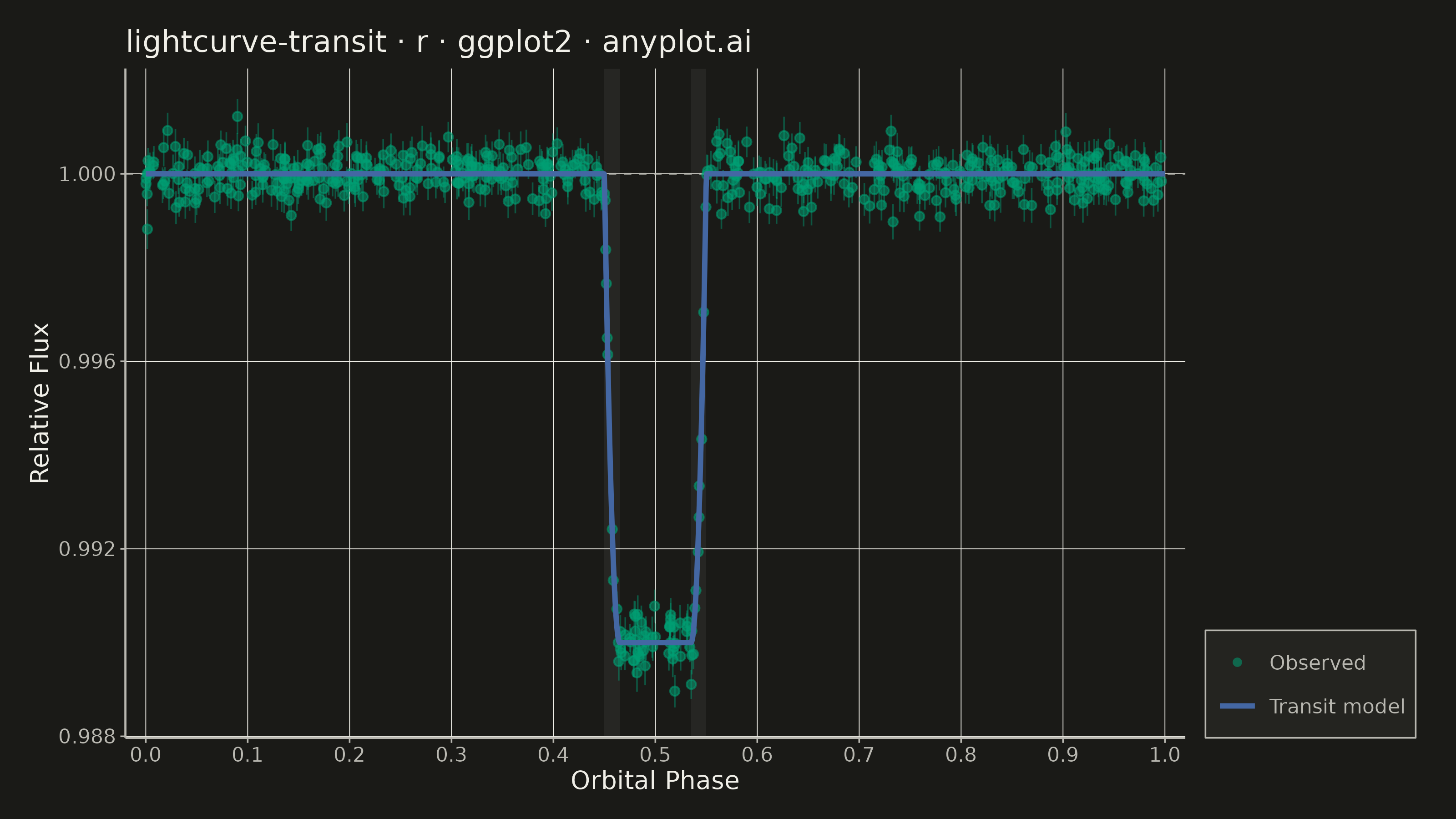
A time-series plot showing the brightness of an astronomical object over time, designed to reveal exoplanet transit events as characteristic dips in flux. The plot displays photometric measurements with error bars against time or orbital phase, with an optional fitted transit model overlay. This visualization is fundamental in observational astronomy for detecting and characterizing planetary transits, variable stars, and other periodic brightness variations.
#' anyplot.ai
#' lightcurve-transit: Astronomical Light Curve
#' Library: ggplot2 3.5.1 | R 4.4.1
#' Quality: 90/100 | Created: 2026-06-20

library(ggplot2)
library(ragg)

set.seed(42)

# Theme tokens (Imprint palette — see prompts/default-style-guide.md)
THEME       <- Sys.getenv("ANYPLOT_THEME", "light")
PAGE_BG     <- if (THEME == "light") "#FAF8F1" else "#1A1A17"
ELEVATED_BG <- if (THEME == "light") "#FFFDF6" else "#242420"
INK         <- if (THEME == "light") "#1A1A17" else "#F0EFE8"
INK_SOFT    <- if (THEME == "light") "#4A4A44" else "#B8B7B0"

IMPRINT_PALETTE <- c(
  "#009E73",  # 1 — brand green (observed data — always first series)
  "#C475FD",  # 2 — lavender
  "#4467A3",  # 3 — blue (transit model)
  "#BD8233",  # 4 — ochre
  "#AE3030",  # 5 — matte red
  "#2ABCCD",  # 6 — cyan
  "#954477",  # 7 — rose
  "#99B314"   # 8 — lime
)

# Transit parameters (shared between data generation and plot annotations)
TRANSIT_CENTER     <- 0.5
TRANSIT_HALF_FLAT  <- 0.035  # half-duration of flat bottom (phase units)
TRANSIT_HALF_TOTAL <- 0.050  # half-duration including ingress/egress
TRANSIT_DEPTH      <- 0.01   # 1% transit depth

# Data: simulated phase-folded exoplanet transit (600 observations)
# Scenario: Hot Jupiter analog with ~1% transit depth, period ~3.5 days
n_obs     <- 600
phase_obs <- runif(n_obs, 0, 1)

# Transit model: flat-bottom shape with smooth quadratic ingress/egress
transit_flux <- function(ph) {
  dp <- ph - TRANSIT_CENTER
  t  <- abs(dp)
  ifelse(
    t <= TRANSIT_HALF_FLAT,
    1.0 - TRANSIT_DEPTH,
    ifelse(
      t <= TRANSIT_HALF_TOTAL,
      1.0 - TRANSIT_DEPTH * (1 - ((t - TRANSIT_HALF_FLAT) / (TRANSIT_HALF_TOTAL - TRANSIT_HALF_FLAT))^2),
      1.0
    )
  )
}

model_vals <- transit_flux(phase_obs)
flux_err   <- abs(rnorm(n_obs, mean = 0.00035, sd = 0.00004))
flux_obs   <- model_vals + rnorm(n_obs, 0, 0.00035)

obs_df <- data.frame(
  phase    = phase_obs,
  flux     = flux_obs,
  flux_err = flux_err
)

# Dense smooth model curve for overlay
phase_grid <- seq(0, 1, length.out = 2000)
model_df   <- data.frame(phase = phase_grid, flux = transit_flux(phase_grid))

# Plot
plot_title <- "lightcurve-transit · r · ggplot2 · anyplot.ai"

p <- ggplot() +
  # Ingress/egress shading via annotate() — transit contact points T1-T4
  annotate(
    "rect",
    xmin  = c(TRANSIT_CENTER - TRANSIT_HALF_TOTAL, TRANSIT_CENTER + TRANSIT_HALF_FLAT),
    xmax  = c(TRANSIT_CENTER - TRANSIT_HALF_FLAT,  TRANSIT_CENTER + TRANSIT_HALF_TOTAL),
    ymin  = -Inf, ymax = Inf,
    fill  = INK_SOFT, alpha = 0.08
  ) +
  # Out-of-transit baseline reference
  geom_hline(
    yintercept = 1.0,
    color      = INK_SOFT,
    linetype   = "dashed",
    linewidth  = 0.35,
    alpha      = 0.7
  ) +
  geom_errorbar(
    data = obs_df,
    aes(x = phase, ymin = flux - flux_err, ymax = flux + flux_err),
    color     = IMPRINT_PALETTE[1],
    width     = 0,
    alpha     = 0.45,
    linewidth = 0.3
  ) +
  geom_point(
    data = obs_df,
    aes(x = phase, y = flux, color = "Observed"),
    size  = 1.4,
    alpha = 0.55
  ) +
  geom_line(
    data = model_df,
    aes(x = phase, y = flux, color = "Transit model"),
    linewidth = 1.0
  ) +
  scale_color_manual(
    name   = NULL,
    values = c("Observed" = IMPRINT_PALETTE[1], "Transit model" = IMPRINT_PALETTE[3])
  ) +
  guides(
    color = guide_legend(
      override.aes = list(
        shape    = c(16, NA),
        linetype = c("blank", "solid")
      )
    )
  ) +
  scale_x_continuous(
    name   = "Orbital Phase",
    breaks = seq(0, 1, by = 0.1),
    expand = c(0.01, 0.01)
  ) +
  scale_y_continuous(
    name   = "Relative Flux",
    labels = function(x) sprintf("%.3f", x)
  ) +
  labs(title = plot_title) +
  theme_minimal(base_size = 8) +
  theme(
    plot.background        = element_rect(fill = PAGE_BG,     color = PAGE_BG),
    panel.background       = element_rect(fill = PAGE_BG,     color = NA),
    panel.grid.major       = element_line(color = INK,        linewidth = 0.15),
    panel.grid.minor       = element_blank(),
    panel.border           = element_blank(),
    axis.line              = element_line(color = INK_SOFT,   linewidth = 0.4),
    axis.ticks             = element_line(color = INK_SOFT,   linewidth = 0.3),
    axis.title             = element_text(color = INK,        size = 10),
    axis.text              = element_text(color = INK_SOFT,   size = 8),
    plot.title             = element_text(color = INK,        size = 12, hjust = 0),
    legend.background      = element_rect(fill = ELEVATED_BG, color = INK_SOFT, linewidth = 0.3),
    legend.text            = element_text(color = INK_SOFT,   size = 8),
    legend.position.inside = c(0.99, 0.04),
    legend.justification   = c("right", "bottom"),
    plot.margin            = margin(12, 16, 10, 12)
  )

# Save
ggsave(
  filename = sprintf("plot-%s.png", THEME),
  plot     = p,
  device   = ragg::agg_png,
  width    = 8,
  height   = 4.5,
  units    = "in",
  dpi      = 400
)
Runnable source as JSON, for any HTTP client: https://api.anyplot.ai/specs/lightcurve-transit/ggplot2/code. Any spec id and library id listed in llms-full.txt fit the same URL shape; every URL below is complete and callable.
{
  "spec_id": "lightcurve-transit",
  "language": "r",
  "library": "ggplot2",
  "page": "https://anyplot.ai/lightcurve-transit/r/ggplot2",
  "hub": "https://anyplot.ai/lightcurve-transit",
  "code_json": "https://api.anyplot.ai/specs/lightcurve-transit/ggplot2/code",
  "spec_json": "https://api.anyplot.ai/specs/lightcurve-transit",
  "render_light_png": "https://storage.googleapis.com/anyplot-images/plots/lightcurve-transit/r/ggplot2/plot-light.png",
  "render_dark_png": "https://storage.googleapis.com/anyplot-images/plots/lightcurve-transit/r/ggplot2/plot-dark.png",
  "quality_score": 90.0,
  "license": "MIT",
  "guide": "https://anyplot.ai/llms.txt"
}
Part of Astronomical Light Curve on anyplot.ai.