The same plot in 14 other libraries — Python: Altair, Bokeh, lets-plot, Matplotlib, Plotly, plotnine, Pygal, Seaborn; Julia: Makie.jl; JavaScript: Chart.js, D3.js, Apache ECharts, Highcharts, MUI X Charts. Compare all 15 side by side: Line Plot with Confidence Interval in Python, R, Julia and JavaScript.
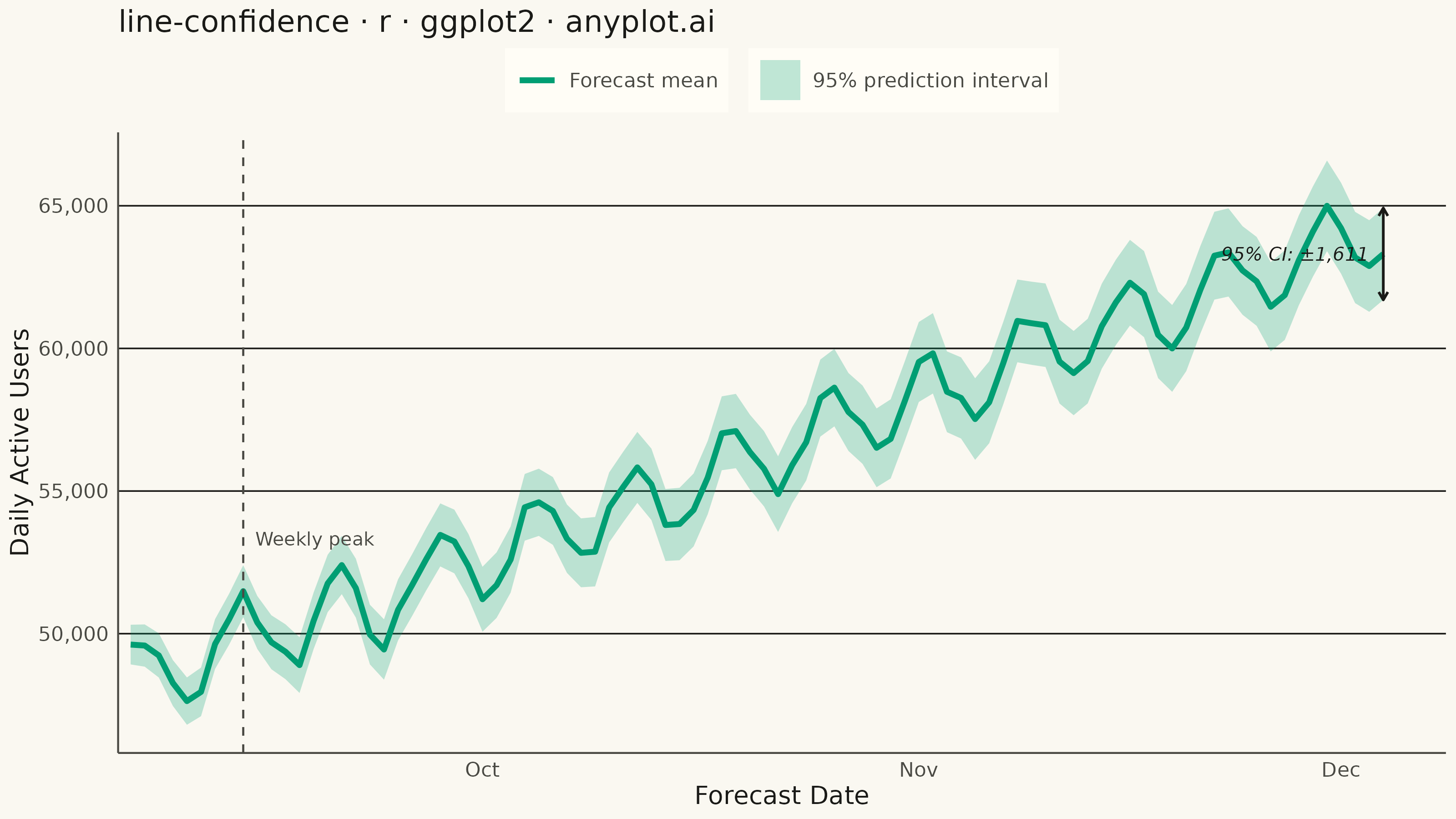
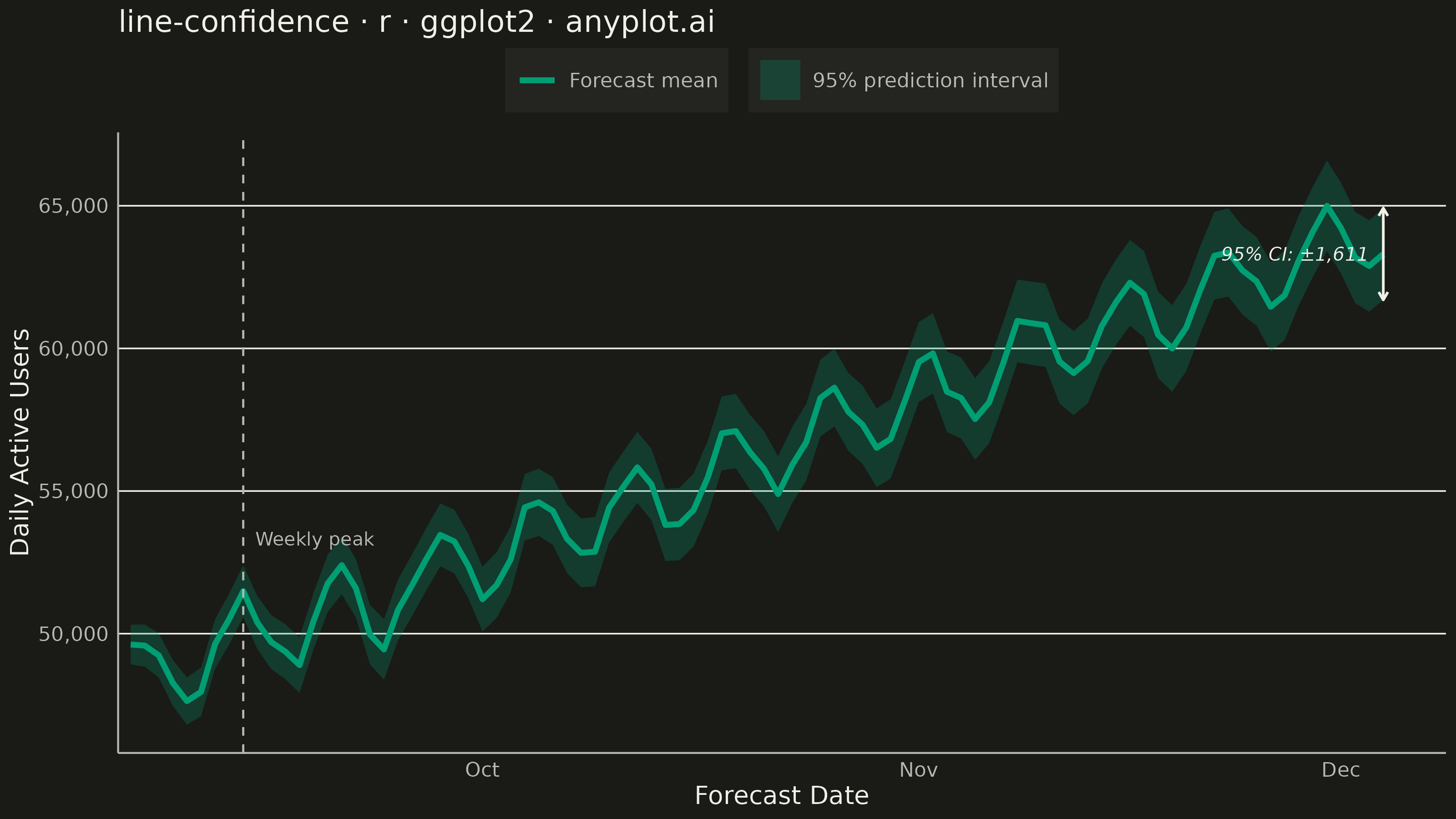
A line plot with a confidence interval displays a central trend line (typically mean or median) surrounded by a shaded band representing uncertainty or variability. The combination of a clear central line and semi-transparent confidence region effectively communicates both the estimated value and its associated uncertainty, making it essential for visualizing statistical estimates, model predictions, and forecast ranges.
#' anyplot.ai
#' line-confidence: Line Plot with Confidence Interval
#' Library: ggplot2 3.5.1 | R 4.4.1
#' Quality: 91/100 | Created: 2026-09-05

library(ggplot2)
library(tibble)
library(scales)
library(ragg)

set.seed(42)

# --- Theme tokens ------------------------------------------------------------
THEME       <- Sys.getenv("ANYPLOT_THEME", "light")
PAGE_BG     <- if (THEME == "light") "#FAF8F1" else "#1A1A17"
ELEVATED_BG <- if (THEME == "light") "#FFFDF6" else "#242420"
INK         <- if (THEME == "light") "#1A1A17" else "#F0EFE8"
INK_SOFT    <- if (THEME == "light") "#4A4A44" else "#B8B7B0"
IMPRINT_PALETTE <- c("#009E73", "#C475FD", "#4467A3", "#BD8233",
                     "#AE3030", "#2ABCCD", "#954477", "#99B314")
BRAND <- IMPRINT_PALETTE[1]

# --- Data ---------------------------------------------------------------------
# 90-day daily-active-user forecast: growth trend plus weekly seasonality,
# with a 95% prediction interval that widens with the forecast horizon
# (sqrt-of-horizon growth, the standard random-walk-forecast uncertainty shape).
horizon_days <- 90
horizon <- seq_len(horizon_days)
forecast_dates <- as.Date("2026-09-05") + horizon

trend <- 48000 + 180 * horizon
seasonality <- 1400 * sin(2 * pi * horizon / 7)
noise <- rnorm(horizon_days, mean = 0, sd = 250)
dau_forecast <- trend + seasonality + noise

standard_error <- 300 + 55 * sqrt(horizon)
dau_lower <- dau_forecast - 1.96 * standard_error
dau_upper <- dau_forecast + 1.96 * standard_error

df <- tibble(
  date  = forecast_dates,
  dau   = dau_forecast,
  lower = dau_lower,
  upper = dau_upper
)

# --- Narrative anchors ------------------------------------------------------
# Weekly seasonality peak (first cycle) - gives viewers a concrete landmark
# for the sawtooth pattern instead of leaving it purely implicit. The label
# sits just above the peak's own ribbon (not the chart's global max) so it
# stays visually anchored to the point it describes.
peak_row  <- df[which.max(df$dau[1:14]), ]
y_span    <- diff(range(c(df$lower, df$upper)))
peak_label_y <- peak_row$upper + y_span * 0.035

# Final-horizon interval width - turns "the band widens" into a concrete
# number, anchoring the growing-uncertainty story at the point it matters most.
last_row   <- df[horizon_days, ]
half_width <- (last_row$upper - last_row$lower) / 2

# --- Plot -----------------------------------------------------------------------
p <- ggplot(df, aes(x = date)) +
  geom_ribbon(aes(ymin = lower, ymax = upper, fill = "95% prediction interval"),
              alpha = 0.25) +
  geom_line(aes(y = dau, color = "Forecast mean"), linewidth = 1.1) +
  geom_vline(xintercept = peak_row$date, linetype = "dashed",
             color = INK_SOFT, linewidth = 0.4) +
  annotate("text", x = peak_row$date, y = peak_label_y, label = "Weekly peak",
           hjust = -0.1, vjust = 0, size = 2.6, color = INK_SOFT) +
  geom_segment(data = last_row,
               aes(x = date, xend = date, y = lower, yend = upper),
               inherit.aes = FALSE, color = INK, linewidth = 0.5,
               arrow = grid::arrow(ends = "both", length = grid::unit(0.05, "in"))) +
  annotate("text", x = last_row$date, y = (last_row$lower + last_row$upper) / 2,
           label = sprintf("95%% CI: ±%s", comma(round(half_width))),
           hjust = 1.1, vjust = 0.5, size = 2.6, color = INK, fontface = "italic") +
  scale_fill_manual(name = NULL, values = c("95% prediction interval" = BRAND)) +
  scale_color_manual(name = NULL, values = c("Forecast mean" = BRAND)) +
  scale_x_date(expand = expansion(mult = c(0.01, 0.05))) +
  scale_y_continuous(labels = label_comma()) +
  coord_cartesian(clip = "off") +
  labs(
    title = "line-confidence · r · ggplot2 · anyplot.ai",
    x = "Forecast Date",
    y = "Daily Active Users"
  ) +
  theme_minimal(base_size = 8) +
  theme(
    plot.background    = element_rect(fill = PAGE_BG, color = PAGE_BG),
    panel.background   = element_rect(fill = PAGE_BG, color = NA),
    panel.grid.major.x = element_blank(),
    panel.grid.major.y = element_line(color = INK, linewidth = 0.3),
    panel.grid.minor   = element_blank(),
    panel.border       = element_blank(),
    axis.title         = element_text(color = INK, size = 10),
    axis.text          = element_text(color = INK_SOFT, size = 8),
    axis.ticks         = element_blank(),
    axis.line          = element_line(color = INK_SOFT),
    plot.title         = element_text(color = INK, size = 12),
    legend.position    = "top",
    legend.background  = element_rect(fill = ELEVATED_BG, color = NA),
    legend.key         = element_rect(fill = ELEVATED_BG, color = NA),
    legend.text        = element_text(color = INK_SOFT, size = 8)
  )

# --- Save -----------------------------------------------------------------------
ggsave(
  filename = sprintf("plot-%s.png", THEME),
  plot     = p,
  device   = ragg::agg_png,
  width    = 8,
  height   = 4.5,
  units    = "in",
  dpi      = 400
)
Runnable source as JSON, for any HTTP client: https://api.anyplot.ai/specs/line-confidence/ggplot2/code. Any spec id and library id listed in llms-full.txt fit the same URL shape; every URL below is complete and callable.
{
  "spec_id": "line-confidence",
  "language": "r",
  "library": "ggplot2",
  "page": "https://anyplot.ai/line-confidence/r/ggplot2",
  "hub": "https://anyplot.ai/line-confidence",
  "code_json": "https://api.anyplot.ai/specs/line-confidence/ggplot2/code",
  "spec_json": "https://api.anyplot.ai/specs/line-confidence",
  "render_light_png": "https://storage.googleapis.com/anyplot-images/plots/line-confidence/r/ggplot2/plot-light.png",
  "render_dark_png": "https://storage.googleapis.com/anyplot-images/plots/line-confidence/r/ggplot2/plot-dark.png",
  "quality_score": 91.0,
  "license": "MIT",
  "guide": "https://anyplot.ai/llms.txt"
}
Part of Line Plot with Confidence Interval on anyplot.ai.