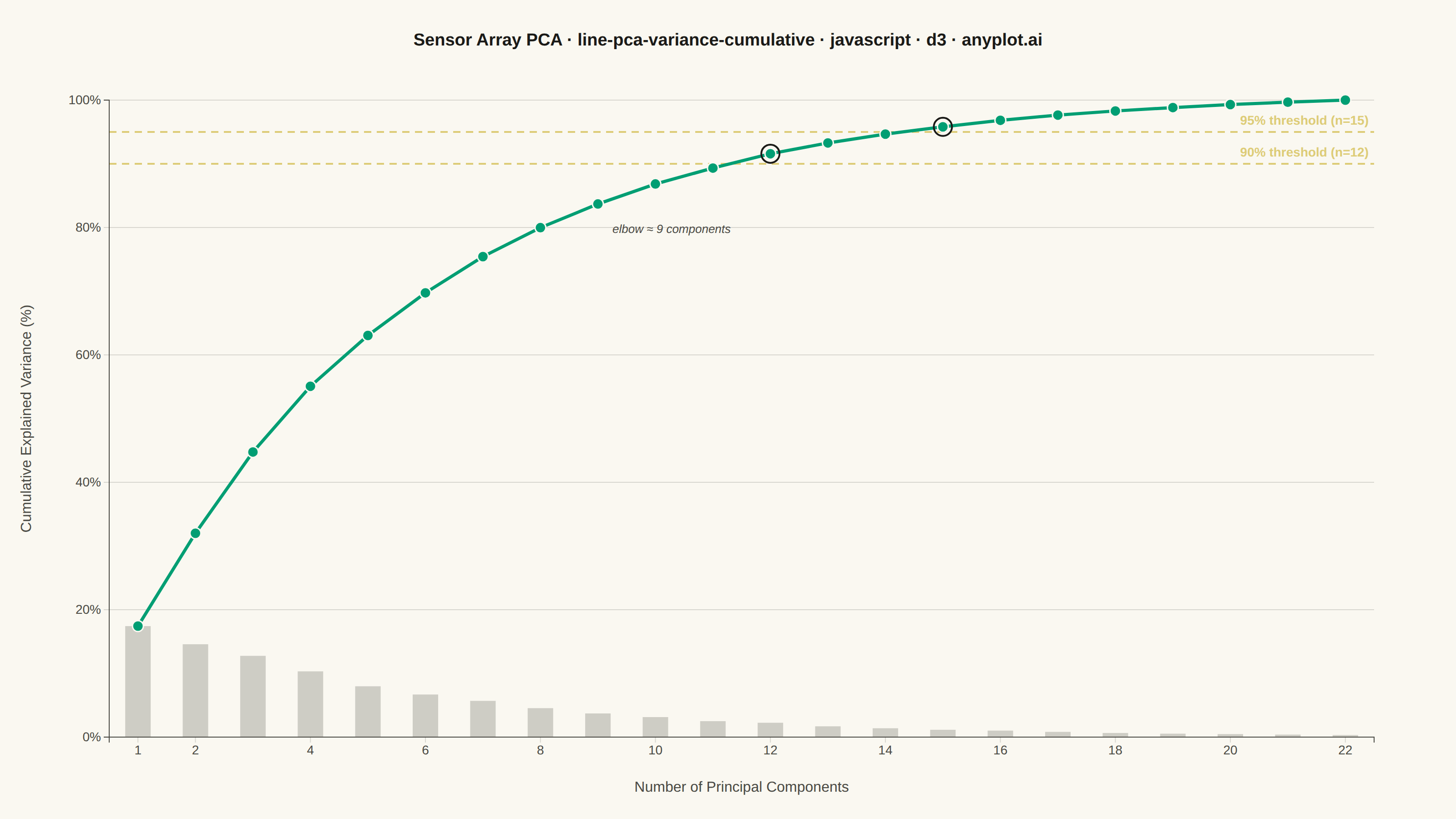
The same plot in 14 other libraries — JavaScript: Chart.js, Apache ECharts, Highcharts, MUI X Charts; Python: Altair, Bokeh, lets-plot, Matplotlib, Plotly, plotnine, Pygal, Seaborn; R: ggplot2; Julia: Makie.jl. Compare all 15 side by side: Cumulative Explained Variance for PCA Component Selection in Python, R, Julia and JavaScript.
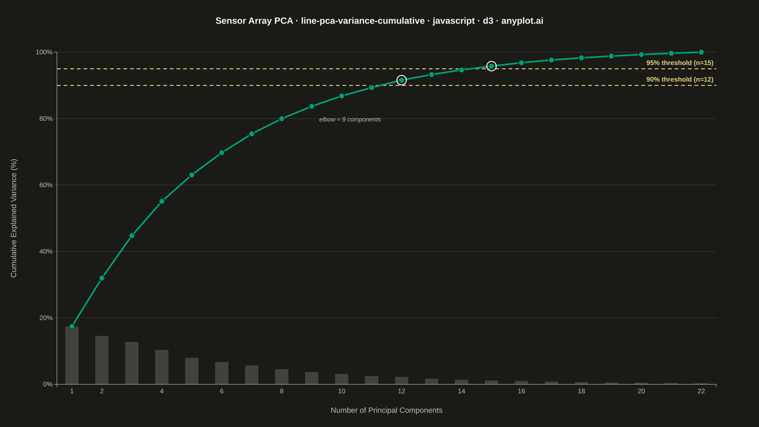
A line plot showing the cumulative proportion of explained variance as a function of the number of Principal Component Analysis (PCA) components. This visualization helps determine the optimal number of components to retain by displaying the trade-off between dimensionality reduction and information preservation. The cumulative curve typically exhibits an elbow pattern where additional components yield diminishing returns, and horizontal threshold lines (e.g., 90%, 95%) guide component selection decisions.
// anyplot.ai
// line-pca-variance-cumulative: Cumulative Explained Variance for PCA Component Selection
// Library: d3 7.9.0 | JavaScript 22.23.2
// Quality: 93/100 | Created: 2026-08-26

const t = window.ANYPLOT_TOKENS;
const { width, height } = window.ANYPLOT_SIZE;
const margin = { top: 110, right: 90, bottom: 90, left: 120 };
const iw = width - margin.left - margin.right;
const ih = height - margin.top - margin.bottom;

// --- Data (in-memory, deterministic) ----------------------------------------
// Synthetic PCA spectrum for a 22-channel industrial sensor array: variance
// concentrates in the first few components (correlated sensor groups), then
// decays with diminishing returns per added component — the classic PCA
// "elbow" shape.
let seed = 20260826;
function lcg() {
  seed = (seed * 1664525 + 1013904223) % 4294967296;
  return seed / 4294967296;
}

const nComponents = 22;
const rawEigenvalues = Array.from({ length: nComponents }, (_, i) => {
  const decay = Math.exp(-i / 5.2);
  const noise = 1 + (lcg() - 0.5) * 0.12;
  return Math.max(decay * noise, 0.002);
});
const eigenvalueSum = d3.sum(rawEigenvalues);
const individualRatio = rawEigenvalues.map((v) => (v / eigenvalueSum) * 100);
const cumulativeRatio = individualRatio.map((_, i) => d3.sum(individualRatio.slice(0, i + 1)));
const componentCounts = d3.range(1, nComponents + 1);

// --- Threshold crossings (first component count reaching each target) --------
const thresholds = [90, 95];
const crossings = thresholds.map((pct) => ({
  pct,
  n: componentCounts[cumulativeRatio.findIndex((v) => v >= pct)],
}));

// --- Elbow detection ------------------------------------------------------------
// Kneedle heuristic: the scree point with the largest perpendicular distance
// from the chord connecting the first and last individual-variance values.
const p1 = { x: 1, y: individualRatio[0] };
const p2 = { x: nComponents, y: individualRatio[nComponents - 1] };
const chordLen = Math.hypot(p2.x - p1.x, p2.y - p1.y);
let elbowIdx = 0;
let maxDist = -Infinity;
individualRatio.forEach((v, i) => {
  const x0 = i + 1;
  const dist = Math.abs((p2.y - p1.y) * x0 - (p2.x - p1.x) * v + p2.x * p1.y - p2.y * p1.x) / chordLen;
  if (dist > maxDist) {
    maxDist = dist;
    elbowIdx = i;
  }
});
const elbowN = elbowIdx + 1;

// --- SVG mount ----------------------------------------------------------------
const svg = d3.select("#container").append("svg").attr("width", width).attr("height", height);
const g = svg.append("g").attr("transform", `translate(${margin.left},${margin.top})`);

// --- Scales ---------------------------------------------------------------------
// Half-unit padding on the x domain keeps the scree bars off the axis edges.
const x = d3.scaleLinear().domain([0.5, nComponents + 0.5]).range([0, iw]);
const y = d3.scaleLinear().domain([0, 100]).range([ih, 0]);

// --- Gridlines (y-axis only) ----------------------------------------------------
g.append("g")
  .attr("class", "grid")
  .call(d3.axisLeft(y).ticks(6).tickSize(-iw).tickFormat(""))
  .call((sel) => sel.select(".domain").remove())
  .selectAll("line")
  .attr("stroke", t.grid);

// --- Individual variance (scree) bars — muted secondary encoding ---------------
const barWidth = Math.min(28, (iw / nComponents) * 0.55);
g.selectAll("rect.scree")
  .data(individualRatio)
  .join("rect")
  .attr("class", "scree")
  .attr("x", (d, i) => x(i + 1) - barWidth / 2)
  .attr("y", (d) => y(d))
  .attr("width", barWidth)
  .attr("height", (d) => ih - y(d))
  .attr("fill", t.inkSoft)
  .attr("opacity", 0.25);

// --- Threshold reference lines (label folds in the crossing count so it
// doesn't need a second floating label that could collide with the curve) --
thresholds.forEach((pct) => {
  const crossN = crossings.find((c) => c.pct === pct).n;

  g.append("line")
    .attr("x1", 0)
    .attr("x2", iw)
    .attr("y1", y(pct))
    .attr("y2", y(pct))
    .attr("stroke", t.amber)
    .attr("stroke-width", 2)
    .attr("stroke-dasharray", "8,6");

  g.append("text")
    .attr("x", iw - 6)
    .attr("y", y(pct) - 8)
    .attr("text-anchor", "end")
    .attr("fill", t.amber)
    .style("font-size", "14px")
    .style("font-weight", "600")
    .text(`${pct}% threshold (n=${crossN})`);
});

// --- Cumulative variance line -----------------------------------------------------
const line = d3
  .line()
  .x((d, i) => x(componentCounts[i]))
  .y((d) => y(d));

g.append("path")
  .datum(cumulativeRatio)
  .attr("fill", "none")
  .attr("stroke", t.palette[0])
  .attr("stroke-width", 3.5)
  .attr("d", line);

// --- Markers at each discrete component count -------------------------------------
g.selectAll("circle.point")
  .data(cumulativeRatio)
  .join("circle")
  .attr("class", "point")
  .attr("cx", (d, i) => x(componentCounts[i]))
  .attr("cy", (d) => y(d))
  .attr("r", 6)
  .attr("fill", t.palette[0])
  .attr("stroke", t.pageBg)
  .attr("stroke-width", 1.5);

// --- Threshold-crossing callouts (ring marker; the count itself is labeled
// on the threshold line above, avoiding a second label that could collide
// with the closely-spaced 90%/95% lines) -------------------------------------
crossings.forEach(({ n }) => {
  g.append("circle")
    .attr("cx", x(n))
    .attr("cy", y(cumulativeRatio[n - 1]))
    .attr("r", 10)
    .attr("fill", "none")
    .attr("stroke", t.ink)
    .attr("stroke-width", 2);
});

// --- Elbow annotation -----------------------------------------------------------------
g.append("text")
  .attr("x", x(elbowN) + 16)
  .attr("y", y(cumulativeRatio[elbowIdx]) + 32)
  .attr("fill", t.inkSoft)
  .style("font-size", "13px")
  .style("font-style", "italic")
  .text(`elbow ≈ ${elbowN} components`);

// --- Axes -------------------------------------------------------------------------
const xTickStep = nComponents > 16 ? 2 : 1;
const xAxis = g
  .append("g")
  .attr("transform", `translate(0,${ih})`)
  .call(
    d3
      .axisBottom(x)
      .tickValues(componentCounts.filter((n) => n === 1 || n % xTickStep === 0))
      .tickFormat(d3.format("d")),
  );
const yAxis = g.append("g").call(d3.axisLeft(y).ticks(6).tickFormat((d) => `${d}%`));

for (const ax of [xAxis, yAxis]) {
  ax.selectAll("text").attr("fill", t.inkSoft).style("font-size", "14px");
  ax.selectAll("line").attr("stroke", t.grid);
  ax.select(".domain").attr("stroke", t.inkSoft);
}

// --- Axis labels -------------------------------------------------------------------
g.append("text")
  .attr("x", iw / 2)
  .attr("y", ih + 60)
  .attr("text-anchor", "middle")
  .attr("fill", t.inkSoft)
  .style("font-size", "16px")
  .text("Number of Principal Components");

g.append("text")
  .attr("transform", "rotate(-90)")
  .attr("x", -ih / 2)
  .attr("y", -86)
  .attr("text-anchor", "middle")
  .attr("fill", t.inkSoft)
  .style("font-size", "16px")
  .text("Cumulative Explained Variance (%)");

// --- Title ---------------------------------------------------------------------------
const title = "Sensor Array PCA · line-pca-variance-cumulative · javascript · d3 · anyplot.ai";
const titleFontSize = Math.max(16, Math.round(22 * Math.min(1, 67 / title.length)));
svg
  .append("text")
  .attr("x", width / 2)
  .attr("y", 50)
  .attr("text-anchor", "middle")
  .attr("fill", t.ink)
  .style("font-size", `${titleFontSize}px`)
  .style("font-weight", "600")
  .text(title);
Runnable source as JSON, for any HTTP client: https://api.anyplot.ai/specs/line-pca-variance-cumulative/d3/code. Any spec id and library id listed in llms-full.txt fit the same URL shape; every URL below is complete and callable.
{
  "spec_id": "line-pca-variance-cumulative",
  "language": "javascript",
  "library": "d3",
  "page": "https://anyplot.ai/line-pca-variance-cumulative/javascript/d3",
  "hub": "https://anyplot.ai/line-pca-variance-cumulative",
  "code_json": "https://api.anyplot.ai/specs/line-pca-variance-cumulative/d3/code",
  "spec_json": "https://api.anyplot.ai/specs/line-pca-variance-cumulative",
  "render_light_png": "https://storage.googleapis.com/anyplot-images/plots/line-pca-variance-cumulative/javascript/d3/plot-light.png",
  "render_dark_png": "https://storage.googleapis.com/anyplot-images/plots/line-pca-variance-cumulative/javascript/d3/plot-dark.png",
  "interactive_light_html": "https://storage.googleapis.com/anyplot-images/plots/line-pca-variance-cumulative/javascript/d3/plot-light.html",
  "interactive_dark_html": "https://storage.googleapis.com/anyplot-images/plots/line-pca-variance-cumulative/javascript/d3/plot-dark.html",
  "quality_score": 93.0,
  "license": "MIT",
  "guide": "https://anyplot.ai/llms.txt"
}
Part of Cumulative Explained Variance for PCA Component Selection on anyplot.ai.