The same plot in 14 other libraries — Python: Altair, Bokeh, lets-plot, Matplotlib, Plotly, plotnine, Pygal, Seaborn; R: ggplot2; JavaScript: Chart.js, D3.js, Apache ECharts, Highcharts, MUI X Charts. Compare all 15 side by side: Cumulative Explained Variance for PCA Component Selection in Python, R, Julia and JavaScript.
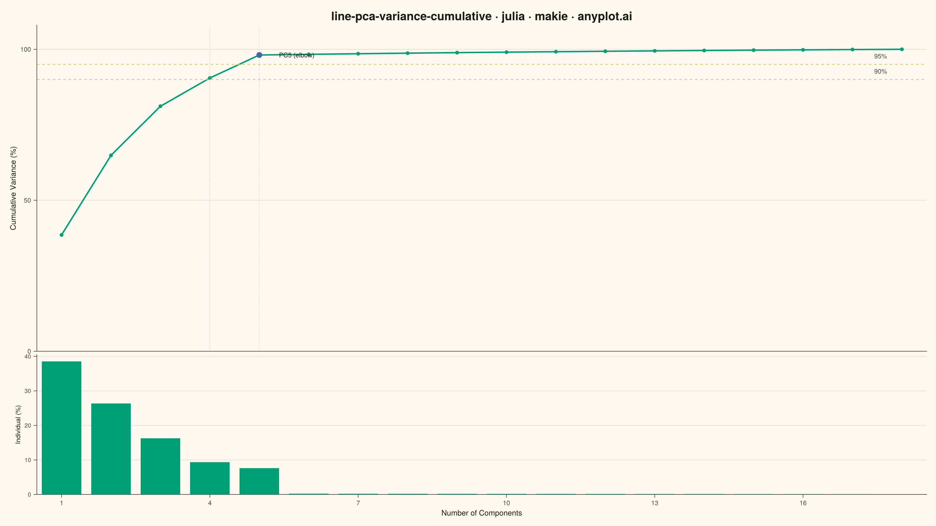
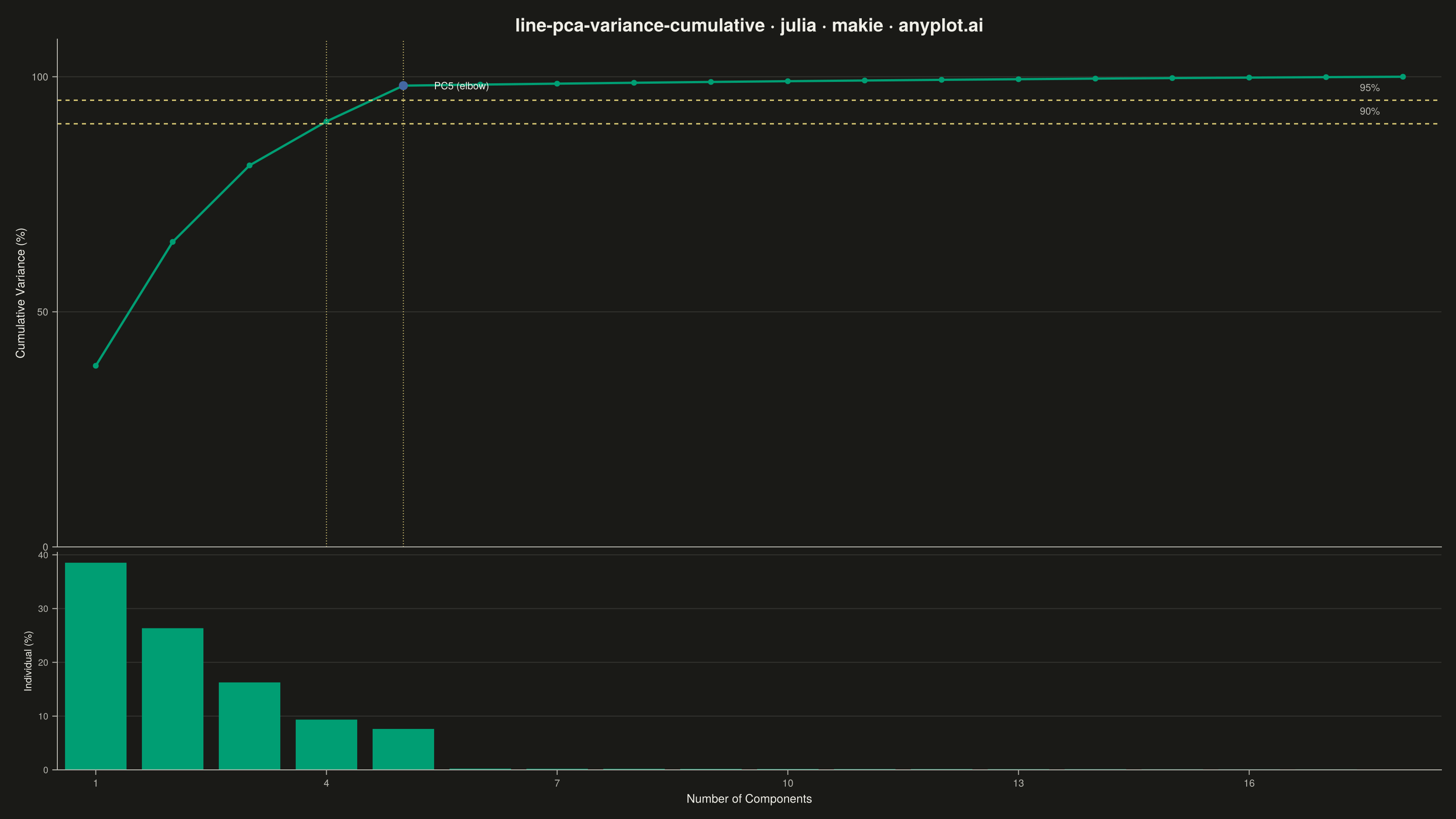
A line plot showing the cumulative proportion of explained variance as a function of the number of Principal Component Analysis (PCA) components. This visualization helps determine the optimal number of components to retain by displaying the trade-off between dimensionality reduction and information preservation. The cumulative curve typically exhibits an elbow pattern where additional components yield diminishing returns, and horizontal threshold lines (e.g., 90%, 95%) guide component selection decisions.
# anyplot.ai
# line-pca-variance-cumulative: Cumulative Explained Variance for PCA Component Selection
# Library: makie 0.22.10 | Julia 1.11.9
# Quality: 89/100 | Created: 2026-05-29

using CairoMakie
using Colors
using Random
using Statistics
using LinearAlgebra

Random.seed!(42)

# Theme tokens — Imprint palette data colors are theme-independent; chrome flips
const THEME       = get(ENV, "ANYPLOT_THEME", "light")
const PAGE_BG     = THEME == "light" ? colorant"#FAF8F1" : colorant"#1A1A17"
const ELEVATED_BG = THEME == "light" ? colorant"#FFFDF6" : colorant"#242420"
const INK         = THEME == "light" ? colorant"#1A1A17" : colorant"#F0EFE8"
const INK_SOFT    = THEME == "light" ? colorant"#4A4A44" : colorant"#B8B7B0"
const INK_MUTED   = THEME == "light" ? colorant"#6B6A63" : colorant"#A8A79F"

const IMPRINT_PALETTE = [
    colorant"#009E73",  # 1 — brand green (always first series)
    colorant"#C475FD",  # 2 — lavender
    colorant"#4467A3",  # 3 — blue
    colorant"#BD8233",  # 4 — ochre
    colorant"#AE3030",  # 5 — matte red
    colorant"#2ABCCD",  # 6 — cyan
    colorant"#954477",  # 7 — rose
    colorant"#99B314",  # 8 — lime
]
const ANYPLOT_AMBER = colorant"#DDCC77"

# Data — synthetic metabolomics dataset: 18 spectral features, 5 true latent factors
n_samples  = 200
n_features = 18

latent   = randn(n_samples, 5)
loadings = randn(5, n_features)
X = latent * loadings .+ 0.4 .* randn(n_samples, n_features)

# PCA via eigendecomposition of the sample covariance matrix
X_c = X .- mean(X, dims=1)
C   = (X_c' * X_c) ./ (n_samples - 1)
eig_result = eigen(Symmetric(C))
eigenvalues = reverse(max.(eig_result.values, 0.0))

evr            = eigenvalues ./ sum(eigenvalues)
cumulative_pct = cumsum(evr) .* 100
individual_pct = evr .* 100
n_comp         = length(eigenvalues)
components     = collect(1:n_comp)

# Elbow: component furthest from the diagonal connecting first and last point
x_n = (components .- 1.0) ./ (n_comp - 1.0)
y_n = (cumulative_pct .- cumulative_pct[1]) ./ (cumulative_pct[end] - cumulative_pct[1])
elbow_idx = argmax(abs.(y_n .- x_n))

idx_90 = something(findfirst(>=(90.0), cumulative_pct), n_comp)
idx_95 = something(findfirst(>=(95.0), cumulative_pct), n_comp)

title_str = "line-pca-variance-cumulative · julia · makie · anyplot.ai"

# Figure — landscape 3200×1800 (resolution=(1600,900) × px_per_unit=2)
fig = Figure(
    size            = (1600, 900),
    fontsize        = 13,
    backgroundcolor = PAGE_BG,
)

ink_grid = RGBAf(INK.r, INK.g, INK.b, 0.12)

# Top panel — cumulative explained variance
ax1 = Axis(
    fig[1, 1];
    title              = title_str,
    titlesize          = 20,
    titlecolor         = INK,
    ylabel             = "Cumulative Variance (%)",
    ylabelsize         = 13,
    ylabelcolor        = INK,
    xticklabelsvisible = false,
    xticksvisible      = false,
    yticklabelsize     = 11,
    yticklabelcolor    = INK_SOFT,
    ytickcolor         = INK_SOFT,
    backgroundcolor    = PAGE_BG,
    topspinevisible    = false,
    rightspinevisible  = false,
    leftspinecolor     = INK_SOFT,
    bottomspinecolor   = INK_SOFT,
    xgridvisible       = false,
    ygridcolor         = ink_grid,
    yminorgridvisible  = false,
    xminorgridvisible  = false,
    limits             = (0.5, n_comp + 0.5, 0.0, 108.0),
)

lines!(ax1, components, cumulative_pct;
    color = IMPRINT_PALETTE[1], linewidth = 2.5)
scatter!(ax1, components, cumulative_pct;
    color = IMPRINT_PALETTE[1], markersize = 9, strokewidth = 0)

hlines!(ax1, [90.0, 95.0];
    color = ANYPLOT_AMBER, linewidth = 1.5, linestyle = :dash)
vlines!(ax1, Float64.([idx_90, idx_95]);
    color = ANYPLOT_AMBER, linewidth = 1.0, linestyle = :dot)

hspan!(ax1, 90.0, 95.0; color = RGBAf(ANYPLOT_AMBER.r, ANYPLOT_AMBER.g, ANYPLOT_AMBER.b, 0.10))

text!(ax1, Float64(n_comp) - 0.3, 91.5;
    text = "90%", color = INK_SOFT, fontsize = 13, align = (:right, :bottom))
text!(ax1, Float64(n_comp) - 0.3, 96.5;
    text = "95%", color = INK_SOFT, fontsize = 13, align = (:right, :bottom))

scatter!(ax1, [Float64(elbow_idx)], [cumulative_pct[elbow_idx]];
    color = IMPRINT_PALETTE[3], markersize = 14, strokewidth = 0)
text!(ax1, Float64(elbow_idx) + 0.4, cumulative_pct[elbow_idx];
    text = "PC$(elbow_idx) (elbow)", color = INK, fontsize = 13,
    align = (:left, :center))

# Bottom panel — individual explained variance bars
ax2 = Axis(
    fig[2, 1];
    xlabel             = "Number of Components",
    ylabel             = "Individual (%)",
    xlabelsize         = 13,
    ylabelsize         = 13,
    xlabelcolor        = INK,
    ylabelcolor        = INK,
    xticklabelcolor    = INK_SOFT,
    yticklabelcolor    = INK_SOFT,
    xtickcolor         = INK_SOFT,
    ytickcolor         = INK_SOFT,
    xticklabelsize     = 11,
    yticklabelsize     = 10,
    backgroundcolor    = PAGE_BG,
    topspinevisible    = false,
    rightspinevisible  = false,
    leftspinecolor     = INK_SOFT,
    bottomspinecolor   = INK_SOFT,
    xgridvisible       = false,
    ygridcolor         = ink_grid,
    yminorgridvisible  = false,
    xminorgridvisible  = false,
    xticks             = 1:3:n_comp,
    limits             = (0.5, n_comp + 0.5, 0.0, nothing),
)

barplot!(ax2, components, individual_pct;
    color = IMPRINT_PALETTE[1], strokewidth = 0)

vlines!(ax2, [Float64(elbow_idx)];
    color = IMPRINT_PALETTE[3], linewidth = 1.5, linestyle = :dash)

linkxaxes!(ax1, ax2)
rowsize!(fig.layout, 1, Relative(0.70))
rowsize!(fig.layout, 2, Relative(0.30))
rowgap!(fig.layout, 1, 6)

save("plot-$(THEME).png", fig; px_per_unit = 2)
Runnable source as JSON, for any HTTP client: https://api.anyplot.ai/specs/line-pca-variance-cumulative/makie/code. Any spec id and library id listed in llms-full.txt fit the same URL shape; every URL below is complete and callable.
{
  "spec_id": "line-pca-variance-cumulative",
  "language": "julia",
  "library": "makie",
  "page": "https://anyplot.ai/line-pca-variance-cumulative/julia/makie",
  "hub": "https://anyplot.ai/line-pca-variance-cumulative",
  "code_json": "https://api.anyplot.ai/specs/line-pca-variance-cumulative/makie/code",
  "spec_json": "https://api.anyplot.ai/specs/line-pca-variance-cumulative",
  "render_light_png": "https://storage.googleapis.com/anyplot-images/plots/line-pca-variance-cumulative/julia/makie/plot-light.png",
  "render_dark_png": "https://storage.googleapis.com/anyplot-images/plots/line-pca-variance-cumulative/julia/makie/plot-dark.png",
  "quality_score": 89.0,
  "license": "MIT",
  "guide": "https://anyplot.ai/llms.txt"
}
Part of Cumulative Explained Variance for PCA Component Selection on anyplot.ai.