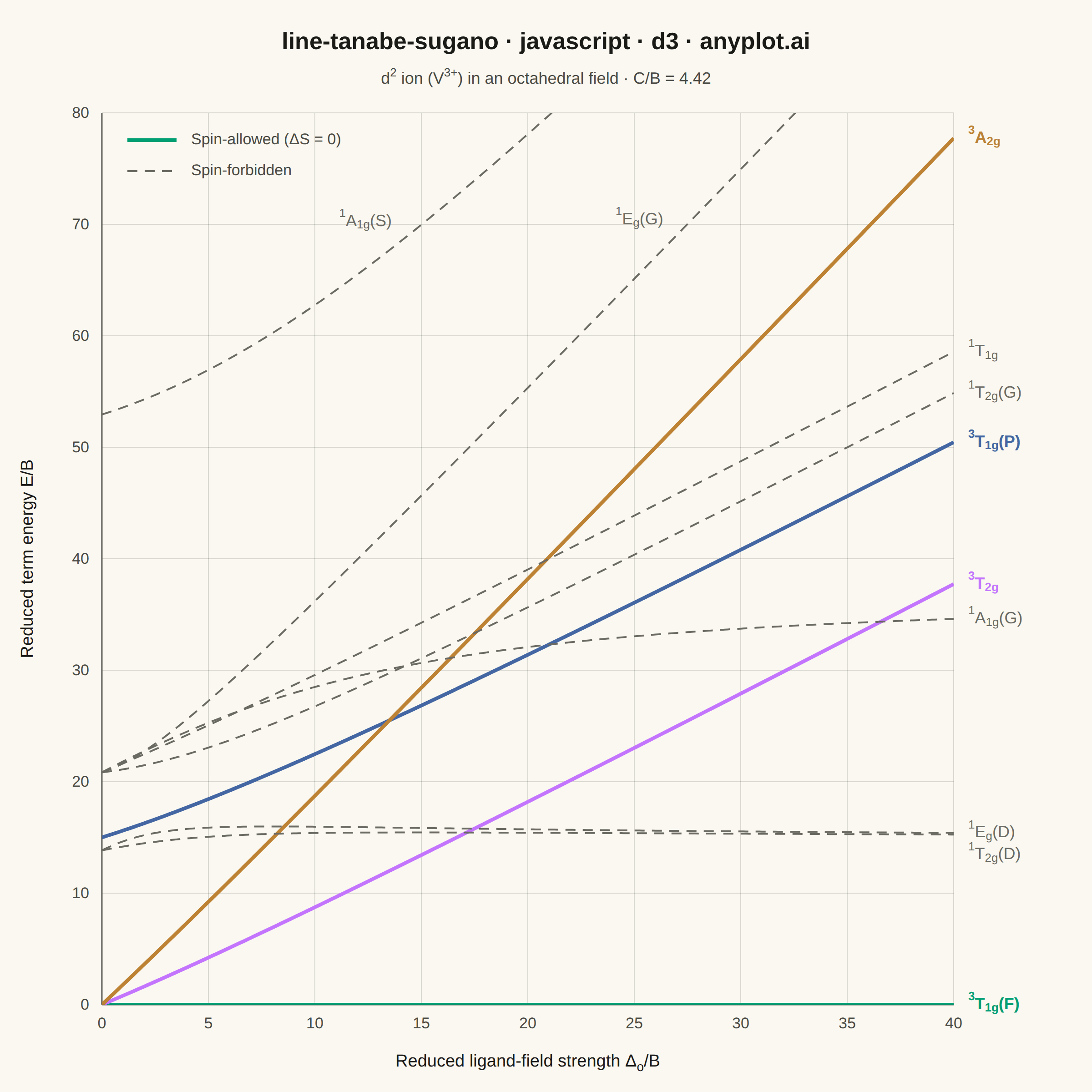
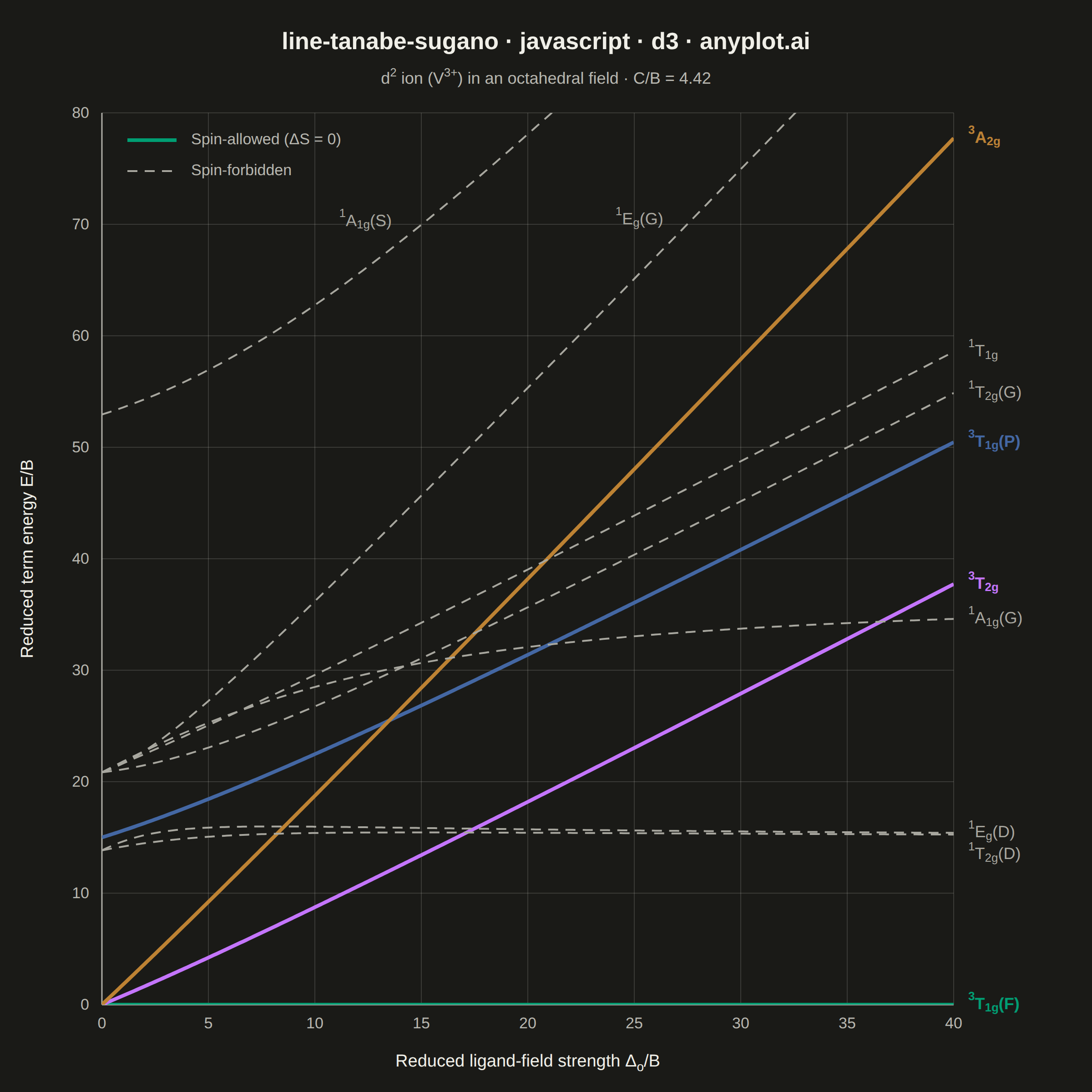
The same plot in 14 other libraries — JavaScript: Chart.js, Apache ECharts, Highcharts, MUI X Charts; Python: Altair, Bokeh, lets-plot, Matplotlib, Plotly, plotnine, Pygal, Seaborn; R: ggplot2; Julia: Makie.jl. Compare all 15 side by side: Tanabe-Sugano Diagram for Crystal Field Theory in Python, R, Julia and JavaScript.
A Tanabe-Sugano diagram plots the energies of the electronic term states of a transition-metal ion in an octahedral ligand field as continuous functions of the field strength. The x-axis is the reduced ligand-field strength Δ_o/B (octahedral splitting divided by the Racah parameter B) and the y-axis is the reduced term energy E/B measured from the ground term, which therefore runs along the x-axis itself as a horizontal line at E/B = 0. Each term — labeled with its full symbol including spin multiplicity and Mulliken label — is one curve, and for d⁴–d⁷ a vertical line marks the high-spin/low-spin crossover where the ground term changes and every curve kinks. Chemists read the chart in reverse: matching ratios of observed UV-Vis band energies against the curves yields both Δ_o and B for a real complex.
// anyplot.ai
// line-tanabe-sugano: Tanabe-Sugano Diagram for Crystal Field Theory
// Library: d3 7.9.0 | JavaScript 22.23.3
// Quality: 90/100 | Created: 2026-10-01
//# anyplot-orientation: square

const t = window.ANYPLOT_TOKENS;
const { width, height } = window.ANYPLOT_SIZE;
const margin = { top: 124, right: 152, bottom: 96, left: 112 };
const iw = width - margin.left - margin.right;
const ih = height - margin.top - margin.bottom;
const FIELD_MAX = 40; // Δ_o/B
const ENERGY_MAX = 80; // E/B
const LABEL_PX = 18;
// Imprint muted anchor — the "rest" class, here the weak spin-forbidden terms.
const MUTED = window.ANYPLOT_THEME === "dark" ? "#A8A79F" : "#6B6A63";

// Term symbols are written in a tiny markup — "^{3}T_{1g}(F)" — and typeset into
// tspans so the multiplicity is a true superscript and the Mulliken index a true
// subscript, instead of printing the plain-text key.
const typeset = (node, markup, px) => {
  let shift = 0;
  for (const [, mark, marked, plain] of markup.matchAll(/([\^_])\{([^}]*)\}|([^\^_]+)/g)) {
    const baseline = mark === "^" ? -0.44 * px : mark === "_" ? 0.26 * px : 0;
    node
      .append("tspan")
      .attr("dy", baseline - shift)
      .attr("font-size", mark ? `${Math.round(px * 0.72)}px` : null)
      .text(mark ? marked : plain);
    shift = baseline;
  }
};

// --- Data: Tanabe-Sugano matrices for d² (V³⁺) at C/B = 4.42 ------------------
// Energies in units of B relative to the Racah A parameter, with q = Dq/B. Every
// term is an eigenvalue of its strong-field block, so terms sharing symmetry and
// multiplicity repel each other instead of crossing — the avoided crossings fall
// out of the algebra. At q = 0 the eigenvalues reduce to the free-ion terms
// (³F −8B, ³P 7B, ¹D −3B+2C, ¹G 4B+2C, ¹S 14B+7C).
const CB = 4.42;
const eigen = (a, b, offDiag) => {
  const centre = (a + b) / 2;
  const spread = Math.hypot((a - b) / 2, offDiag);
  return [centre - spread, centre + spread];
};
const tripletT1 = (q) => eigen(-5 - 12 * q, 4 - 2 * q, 6);
const singletE = (q) => eigen(1 + 2 * CB - 12 * q, 2 * CB + 8 * q, 2 * Math.sqrt(3));
const singletT2 = (q) => eigen(1 + 2 * CB - 12 * q, 2 * CB - 2 * q, 2 * Math.sqrt(3));
const singletA1 = (q) => eigen(10 + 5 * CB - 12 * q, 8 + 4 * CB + 8 * q, Math.sqrt(6) * (2 + CB));

const terms = [
  { symbol: "^{3}T_{1g}(F)", allowed: true, color: t.palette[0], energy: (q) => tripletT1(q)[0] },
  { symbol: "^{3}T_{2g}", allowed: true, color: t.palette[1], energy: (q) => -8 - 2 * q },
  { symbol: "^{3}T_{1g}(P)", allowed: true, color: t.palette[2], energy: (q) => tripletT1(q)[1] },
  { symbol: "^{3}A_{2g}", allowed: true, color: t.palette[3], energy: (q) => -8 + 8 * q },
  { symbol: "^{1}E_{g}(D)", allowed: false, color: MUTED, energy: (q) => singletE(q)[0] },
  { symbol: "^{1}T_{2g}(D)", allowed: false, color: MUTED, energy: (q) => singletT2(q)[0] },
  { symbol: "^{1}T_{1g}", allowed: false, color: MUTED, energy: (q) => 4 + 2 * CB - 2 * q },
  { symbol: "^{1}A_{1g}(G)", allowed: false, color: MUTED, energy: (q) => singletA1(q)[0] },
  { symbol: "^{1}T_{2g}(G)", allowed: false, color: MUTED, energy: (q) => singletT2(q)[1] },
  { symbol: "^{1}E_{g}(G)", allowed: false, color: MUTED, energy: (q) => singletE(q)[1] },
  { symbol: "^{1}A_{1g}(S)", allowed: false, color: MUTED, energy: (q) => singletA1(q)[1] },
];

// Δ_o/B = 10·Dq/B, 321 samples; the ground term ³T₁g(F) is the energy reference,
// so it is a flat curve along E/B = 0.
const field = d3.range(0, FIELD_MAX + 1e-9, 0.125);
const curves = terms.map((term) => ({
  ...term,
  points: field.map((fieldStrength) => ({
    fieldStrength,
    energy: term.energy(fieldStrength / 10) - tripletT1(fieldStrength / 10)[0],
  })),
}));

// --- SVG mount ---------------------------------------------------------------
const svg = d3.select("#container").append("svg").attr("width", width).attr("height", height);
const g = svg.append("g").attr("transform", `translate(${margin.left},${margin.top})`);

// --- Scales ------------------------------------------------------------------
const x = d3.scaleLinear().domain([0, FIELD_MAX]).range([0, iw]);
const y = d3.scaleLinear().domain([0, ENERGY_MAX]).range([ih, 0]);

// --- Grid --------------------------------------------------------------------
g.append("g")
  .selectAll("line")
  .data(x.ticks(8))
  .join("line")
  .attr("x1", x)
  .attr("x2", x)
  .attr("y2", ih)
  .attr("stroke", t.grid);
g.append("g")
  .selectAll("line")
  .data(y.ticks(8))
  .join("line")
  .attr("y1", y)
  .attr("y2", y)
  .attr("x2", iw)
  .attr("stroke", t.grid);

// --- Axes --------------------------------------------------------------------
const xAxis = g
  .append("g")
  .attr("transform", `translate(0,${ih})`)
  .call(d3.axisBottom(x).ticks(8).tickSize(0).tickPadding(14));
const yAxis = g.append("g").call(d3.axisLeft(y).ticks(8).tickSize(0).tickPadding(14));
for (const axis of [xAxis, yAxis]) {
  axis.selectAll("text").attr("fill", t.inkSoft).style("font-size", "17px");
  axis.select(".domain").attr("stroke", t.inkSoft).attr("stroke-width", 1.4);
}

const xLabel = svg
  .append("text")
  .attr("x", margin.left + iw / 2)
  .attr("y", height - 28)
  .attr("text-anchor", "middle")
  .attr("fill", t.ink)
  .style("font-size", "19px");
typeset(xLabel, "Reduced ligand-field strength Δ_{o}/B", 19);
svg
  .append("text")
  .attr("transform", `translate(36,${margin.top + ih / 2}) rotate(-90)`)
  .attr("text-anchor", "middle")
  .attr("fill", t.ink)
  .style("font-size", "19px")
  .text("Reduced term energy E/B");

// --- Term curves: spin-allowed thick and solid, spin-forbidden thin and dashed
svg.append("clipPath").attr("id", "plot-area").append("rect").attr("width", iw).attr("height", ih);
const line = d3
  .line()
  .x((p) => x(p.fieldStrength))
  .y((p) => y(p.energy));
g.append("g")
  .attr("clip-path", "url(#plot-area)")
  .selectAll("path")
  .data(curves)
  .join("path")
  .attr("d", (curve) => line(curve.points))
  .attr("fill", "none")
  .attr("stroke", (curve) => curve.color)
  .attr("stroke-width", (curve) => (curve.allowed ? 4 : 2))
  .attr("stroke-dasharray", (curve) => (curve.allowed ? null : "11 8"));

// --- Term labels at the right edge, or where a curve leaves the top ----------
const labels = curves.map((curve) => {
  const end = curve.points[curve.points.length - 1];
  if (end.energy <= ENERGY_MAX) {
    return { ...curve, atEdge: true, px: iw + 16, py: y(end.energy) };
  }
  // The curve leaves the top of the frame: label it along the curve instead,
  // sitting just above the line where it is still well inside.
  const anchor = curve.points.filter((p) => p.energy <= 0.86 * ENERGY_MAX).pop();
  return {
    ...curve,
    atEdge: false,
    px: x(anchor.fieldStrength) - 12,
    py: y(anchor.energy) - 20,
  };
});
// Where two curves end near-coincident, the labels move apart — the curves stay
// on their data values.
const atEdge = labels.filter((label) => label.atEdge).sort((a, b) => a.py - b.py);
atEdge.forEach((label, i) => {
  if (i > 0) label.py = Math.max(label.py, atEdge[i - 1].py + LABEL_PX + 6);
});
for (const label of labels) {
  const node = svg
    .append("text")
    .attr("x", margin.left + label.px)
    .attr("y", margin.top + label.py)
    .attr("text-anchor", label.atEdge ? "start" : "end")
    .attr("dominant-baseline", "middle")
    .attr("fill", label.color)
    .style("font-size", `${LABEL_PX}px`)
    .style("font-weight", label.allowed ? "600" : "400");
  typeset(node, label.symbol, LABEL_PX);
}

// --- Title, subtitle and the spin-selection key ------------------------------
svg
  .append("text")
  .attr("x", width / 2)
  .attr("y", 54)
  .attr("text-anchor", "middle")
  .attr("fill", t.ink)
  .style("font-size", "26px")
  .style("font-weight", "600")
  .text("line-tanabe-sugano · javascript · d3 · anyplot.ai");
const subtitle = svg
  .append("text")
  .attr("x", width / 2)
  .attr("y", 92)
  .attr("text-anchor", "middle")
  .attr("fill", t.inkSoft)
  .style("font-size", "18px");
typeset(subtitle, "d^{2} ion (V^{3+}) in an octahedral field · C/B = 4.42", 18);

const legend = g.append("g").attr("transform", "translate(28,30)");
const key = [
  { text: "Spin-allowed (ΔS = 0)", color: t.palette[0], dash: null, stroke: 4 },
  { text: "Spin-forbidden", color: MUTED, dash: "11 8", stroke: 2 },
];
key.forEach((entry, i) => {
  legend
    .append("line")
    .attr("x2", 54)
    .attr("y1", i * 34)
    .attr("y2", i * 34)
    .attr("stroke", entry.color)
    .attr("stroke-width", entry.stroke)
    .attr("stroke-dasharray", entry.dash);
  legend
    .append("text")
    .attr("x", 70)
    .attr("y", i * 34)
    .attr("dominant-baseline", "middle")
    .attr("fill", t.inkSoft)
    .style("font-size", "17px")
    .text(entry.text);
});
Runnable source as JSON, for any HTTP client: https://api.anyplot.ai/specs/line-tanabe-sugano/d3/code. Any spec id and library id listed in llms-full.txt fit the same URL shape; every URL below is complete and callable.
{
  "spec_id": "line-tanabe-sugano",
  "language": "javascript",
  "library": "d3",
  "page": "https://anyplot.ai/line-tanabe-sugano/javascript/d3",
  "hub": "https://anyplot.ai/line-tanabe-sugano",
  "code_json": "https://api.anyplot.ai/specs/line-tanabe-sugano/d3/code",
  "spec_json": "https://api.anyplot.ai/specs/line-tanabe-sugano",
  "render_light_png": "https://storage.googleapis.com/anyplot-images/plots/line-tanabe-sugano/javascript/d3/plot-light.png",
  "render_dark_png": "https://storage.googleapis.com/anyplot-images/plots/line-tanabe-sugano/javascript/d3/plot-dark.png",
  "interactive_light_html": "https://storage.googleapis.com/anyplot-images/plots/line-tanabe-sugano/javascript/d3/plot-light.html",
  "interactive_dark_html": "https://storage.googleapis.com/anyplot-images/plots/line-tanabe-sugano/javascript/d3/plot-dark.html",
  "quality_score": 90.0,
  "license": "MIT",
  "guide": "https://anyplot.ai/llms.txt"
}
Part of Tanabe-Sugano Diagram for Crystal Field Theory on anyplot.ai.