The same plot in 14 other libraries — Python: Altair, Bokeh, lets-plot, Matplotlib, Plotly, plotnine, Seaborn; R: ggplot2; Julia: Makie.jl; JavaScript: Chart.js, D3.js, Apache ECharts, Highcharts, MUI X Charts. Compare all 15 side by side: Tanabe-Sugano Diagram for Crystal Field Theory in Python, R, Julia and JavaScript.
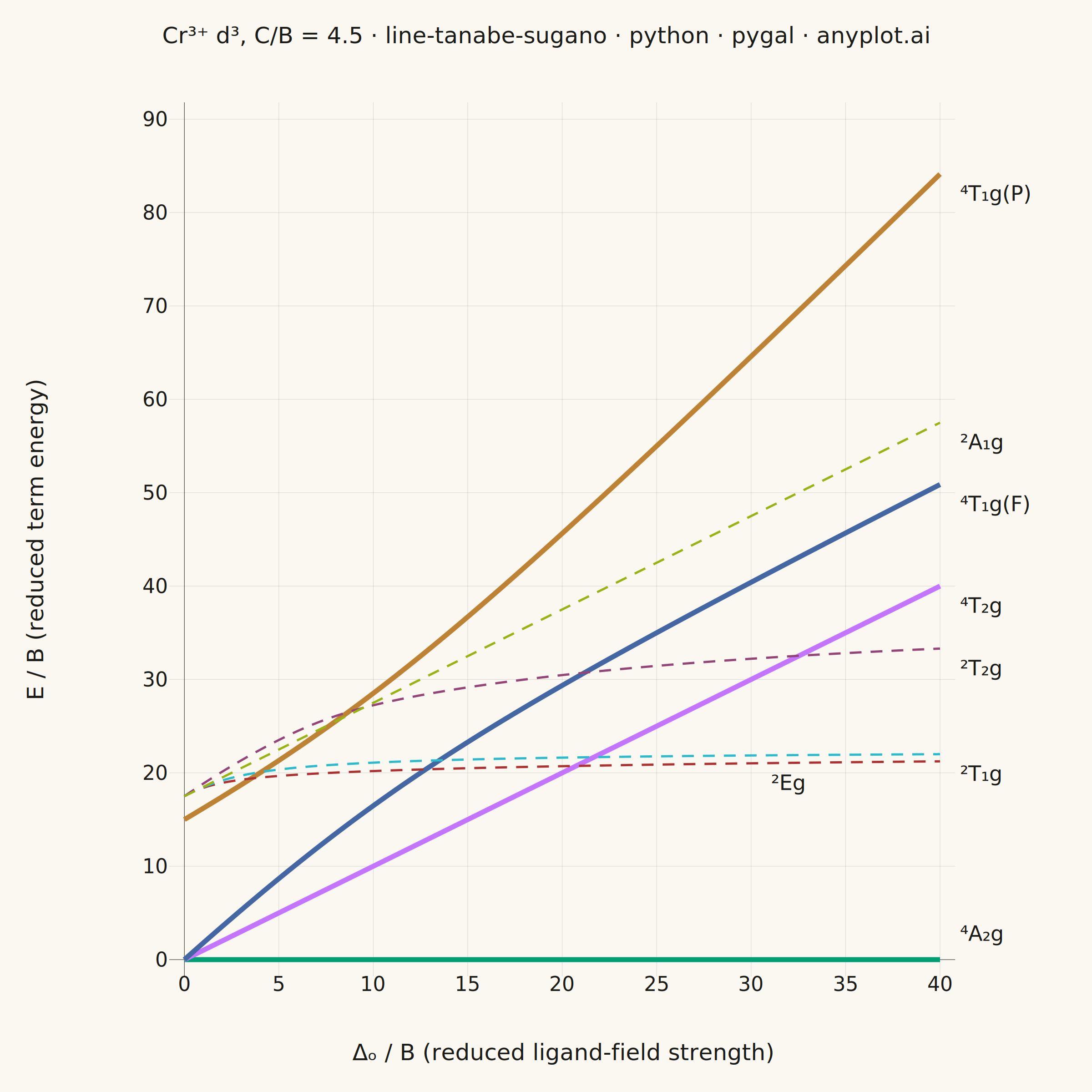
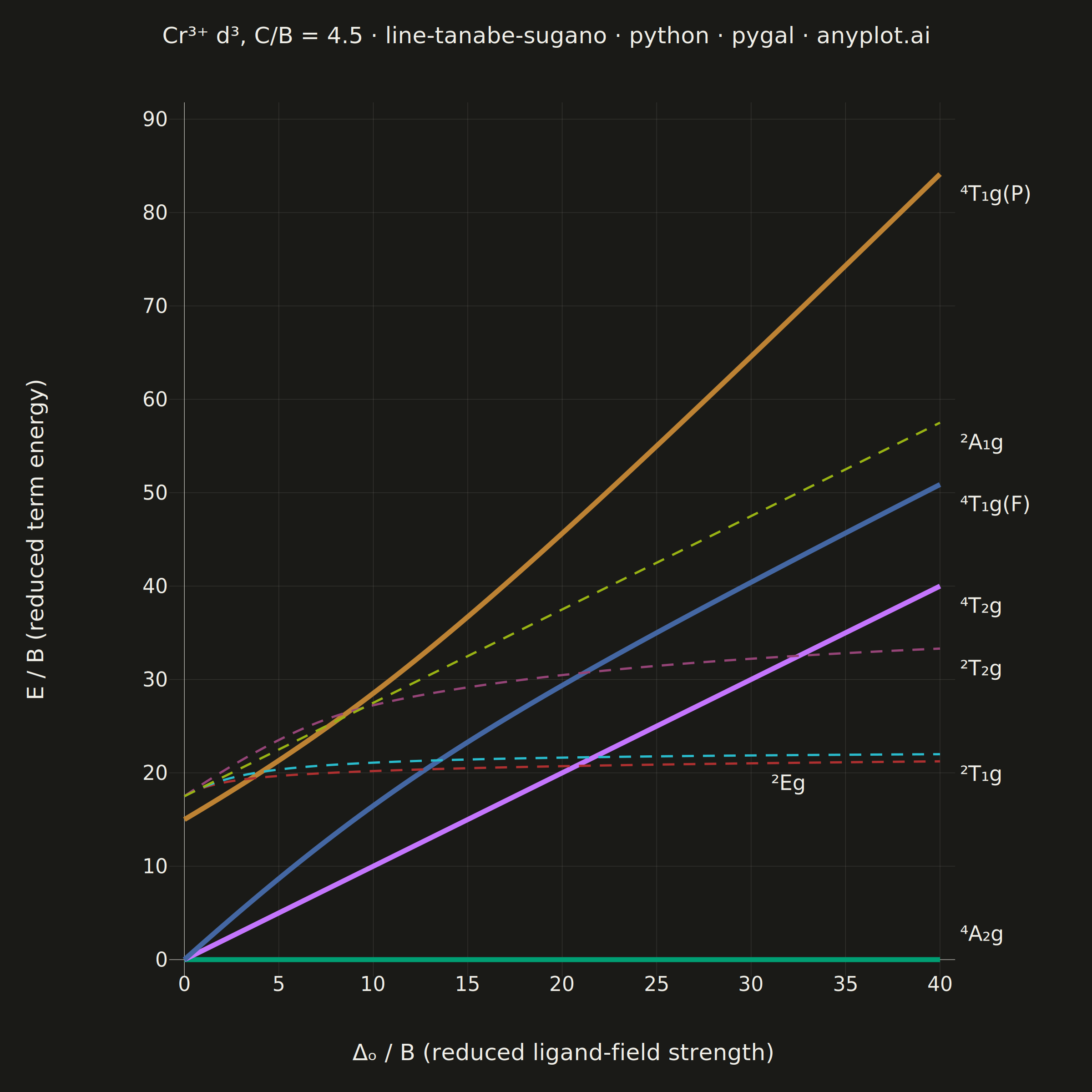
A Tanabe-Sugano diagram plots the energies of the electronic term states of a transition-metal ion in an octahedral ligand field as continuous functions of the field strength. The x-axis is the reduced ligand-field strength Δ_o/B (octahedral splitting divided by the Racah parameter B) and the y-axis is the reduced term energy E/B measured from the ground term, which therefore runs along the x-axis itself as a horizontal line at E/B = 0. Each term — labeled with its full symbol including spin multiplicity and Mulliken label — is one curve, and for d⁴–d⁷ a vertical line marks the high-spin/low-spin crossover where the ground term changes and every curve kinks. Chemists read the chart in reverse: matching ratios of observed UV-Vis band energies against the curves yields both Δ_o and B for a real complex.
""" anyplot.ai
line-tanabe-sugano: Tanabe-Sugano Diagram for Crystal Field Theory
Library: pygal 3.1.3 | Python 3.13.15
Quality: 88/100 | Created: 2026-10-01
"""

import os

import numpy as np
import pygal
from pygal.style import Style


# Theme tokens (see prompts/default-style-guide.md "Theme-adaptive Chrome")
THEME = os.getenv("ANYPLOT_THEME", "light")
PAGE_BG = "#FAF8F1" if THEME == "light" else "#1A1A17"
INK = "#1A1A17" if THEME == "light" else "#F0EFE8"
INK_SOFT = "#4A4A44" if THEME == "light" else "#B8B7B0"
GRID = "rgba(26,26,23,0.15)" if THEME == "light" else "rgba(240,239,232,0.15)"

# Imprint palette — position 1 (#009E73) is always the first series
IMPRINT_PALETTE = ("#009E73", "#C475FD", "#4467A3", "#BD8233", "#AE3030", "#2ABCCD", "#954477", "#99B314")

# Data — d³ (Cr³⁺) in an octahedral field, every energy in units of the Racah
# parameter B, at the textbook ratio C/B = 4.5. The field strength enters as
# Dq/B, with the octahedral splitting Δ_o = 10 Dq.
racah_c = 4.5
delta_over_b = np.linspace(0.0, 40.0, 241)
dq = delta_over_b / 10.0
sqrt2 = np.sqrt(2.0)
sqrt3 = np.sqrt(3.0)

# The ⁴A₂g(t₂g³) ground term; every curve is referenced to it, so it is flat at 0
ground_energy = -12 * dq - 15

# Tanabe-Sugano matrices for d³ (Sugano, Tanabe & Kamimura), one symmetry block
# per entry as its diagonal elements plus the upper-triangle couplings
ts_blocks = {
    "quartet_t1": ([-2 * dq - 3, 8 * dq - 12], {(0, 1): 6}),
    "doublet_e": (
        [-12 * dq - 6 + 3 * racah_c, -2 * dq + 8 + 6 * racah_c, -2 * dq - 1 + 3 * racah_c, 18 * dq - 8 + 4 * racah_c],
        {(0, 1): -6 * sqrt2, (0, 2): -3 * sqrt2, (1, 2): 10, (1, 3): sqrt3 * (2 + racah_c), (2, 3): 2 * sqrt3},
    ),
    "doublet_t1": (
        [
            -12 * dq - 6 + 3 * racah_c,
            -2 * dq + 3 * racah_c,
            -2 * dq - 6 + 3 * racah_c,
            8 * dq - 6 + 3 * racah_c,
            8 * dq - 2 + 3 * racah_c,
        ],
        {
            (0, 1): -3,
            (0, 2): 3,
            (0, 4): -2 * sqrt3,
            (1, 2): -3,
            (1, 3): 3,
            (1, 4): 3 * sqrt3,
            (2, 3): -3,
            (2, 4): -sqrt3,
            (3, 4): 2 * sqrt3,
        },
    ),
    "doublet_t2": (
        [
            -12 * dq + 5 * racah_c,
            -2 * dq - 6 + 3 * racah_c,
            -2 * dq + 4 + 3 * racah_c,
            8 * dq + 6 + 5 * racah_c,
            8 * dq - 2 + 3 * racah_c,
        ],
        {
            (0, 1): -3 * sqrt3,
            (0, 2): -5 * sqrt3,
            (0, 3): 4 + 2 * racah_c,
            (0, 4): 2,
            (1, 2): 3,
            (1, 3): -3 * sqrt3,
            (1, 4): -3 * sqrt3,
            (2, 3): -sqrt3,
            (2, 4): sqrt3,
            (3, 4): 10,
        },
    ),
}

# Diagonalizing each block at every field strength keeps terms of the same symmetry
# and multiplicity as avoided crossings instead of letting them cross
term_energies = {}
for block_name, (diagonal, couplings) in ts_blocks.items():
    block = np.zeros((len(dq), len(diagonal), len(diagonal)))
    for i, element in enumerate(diagonal):
        block[:, i, i] = element
    for (i, j), element in couplings.items():
        block[:, i, j] = block[:, j, i] = element
    term_energies[block_name] = np.linalg.eigvalsh(block) - ground_energy[:, None]

# Term symbol, curve, spin-allowed flag (same multiplicity as ⁴A₂g) and the field
# strength the term label is anchored to. Unicode stands in for sub/superscripts:
# pygal renders plain SVG text with no markup, so the g stays on the baseline.
term_curves = [
    ("⁴A₂g", np.zeros_like(dq), True, 40.0),
    ("⁴T₂g", -2 * dq - 15 - ground_energy, True, 40.0),
    ("⁴T₁g(F)", term_energies["quartet_t1"][:, 0], True, 40.0),
    ("⁴T₁g(P)", term_energies["quartet_t1"][:, 1], True, 40.0),
    ("²Eg", term_energies["doublet_e"][:, 0], False, 30.0),
    ("²T₁g", term_energies["doublet_t1"][:, 0], False, 40.0),
    ("²T₂g", term_energies["doublet_t2"][:, 0], False, 40.0),
    ("²A₁g", -2 * dq - 11 + 3 * racah_c - ground_energy, False, 40.0),
]

# pygal pins stroke-width on every reactive path, hard-codes black label text and drops
# every curve label below its anchor point, so the thin spin-forbidden lines, the
# theme-adaptive label color and the flat ground term's label need one more sheet: at
# E/B = 0 that drop would land ⁴A₂g inside the x-tick row, hence the lift
spin_forbidden_lines = ",".join(
    f".serie-{i} .line" for i, (_, _, spin_allowed, _) in enumerate(term_curves) if not spin_allowed
)
ground_label_lift = ".text-overlay .serie-0 text.label{transform:translate(0px,-100px)}"
extra_css = (
    f"inline:{spin_forbidden_lines}{{stroke-width:5 !important}}"
    f".text-overlay text{{fill:{INK} !important}}{ground_label_lift}"
)

# Plot — square canvas, since the diagram reads best on a near-square plot area
title = "Cr³⁺ d³, C/B = 4.5 · line-tanabe-sugano · python · pygal · anyplot.ai"
custom_style = Style(
    background=PAGE_BG,
    plot_background=PAGE_BG,
    foreground=INK,
    foreground_strong=INK,
    foreground_subtle=INK_SOFT,
    guide_stroke_color=GRID,
    major_guide_stroke_color=GRID,
    guide_stroke_dasharray="none",
    major_guide_stroke_dasharray="none",
    colors=IMPRINT_PALETTE,
    font_family="DejaVu Sans, sans-serif",
    title_font_size=50,
    label_font_size=44,
    major_label_font_size=44,
    value_font_size=44,
    value_label_font_size=46,
    stroke_opacity="1",
    stroke_width=11,
)

chart = pygal.XY(
    # pygal pins the title at title_font_size + spacing from the canvas top, so spacing
    # — not margin_top — is what buys air above it; the margins then centre the plot area
    spacing=45,
    width=2400,
    height=2400,
    style=custom_style,
    css=["file://style.css", "file://graph.css", extra_css],
    title=title,
    x_title="Δₒ / B  (reduced ligand-field strength)",
    y_title="E / B  (reduced term energy)",
    xrange=(0, 40),
    range=(0, 90),
    x_labels=[0, 5, 10, 15, 20, 25, 30, 35, 40],
    y_labels=[0, 10, 20, 30, 40, 50, 60, 70, 80, 90],
    show_x_guides=True,
    show_y_guides=True,
    show_legend=False,
    dots_size=0,
    print_labels=True,
    print_values=False,
    margin_top=130,
    margin_bottom=70,
    margin_left=180,
    margin_right=300,
)

# Style — spin-allowed terms thick and solid, the weak spin-forbidden ones thin and
# dashed; each term symbol is printed next to the sample its own curve passes through
for term, energy, spin_allowed, label_at in term_curves:
    points = list(zip(delta_over_b.tolist(), energy.tolist(), strict=True))
    anchor = int(np.argmin(np.abs(delta_over_b - label_at)))
    points[anchor] = {"value": points[anchor], "label": term}
    chart.add(term, points, stroke_style=None if spin_allowed else {"dasharray": "26, 20"})

# Save
chart.render_to_png(f"plot-{THEME}.png")
chart.render_to_file(f"plot-{THEME}.html")
Runnable source as JSON, for any HTTP client: https://api.anyplot.ai/specs/line-tanabe-sugano/pygal/code. Any spec id and library id listed in llms-full.txt fit the same URL shape; every URL below is complete and callable.
{
  "spec_id": "line-tanabe-sugano",
  "language": "python",
  "library": "pygal",
  "page": "https://anyplot.ai/line-tanabe-sugano/python/pygal",
  "hub": "https://anyplot.ai/line-tanabe-sugano",
  "code_json": "https://api.anyplot.ai/specs/line-tanabe-sugano/pygal/code",
  "spec_json": "https://api.anyplot.ai/specs/line-tanabe-sugano",
  "render_light_png": "https://storage.googleapis.com/anyplot-images/plots/line-tanabe-sugano/python/pygal/plot-light.png",
  "render_dark_png": "https://storage.googleapis.com/anyplot-images/plots/line-tanabe-sugano/python/pygal/plot-dark.png",
  "interactive_light_html": "https://storage.googleapis.com/anyplot-images/plots/line-tanabe-sugano/python/pygal/plot-light.html",
  "interactive_dark_html": "https://storage.googleapis.com/anyplot-images/plots/line-tanabe-sugano/python/pygal/plot-dark.html",
  "quality_score": 88.0,
  "license": "MIT",
  "guide": "https://anyplot.ai/llms.txt"
}
Part of Tanabe-Sugano Diagram for Crystal Field Theory on anyplot.ai.