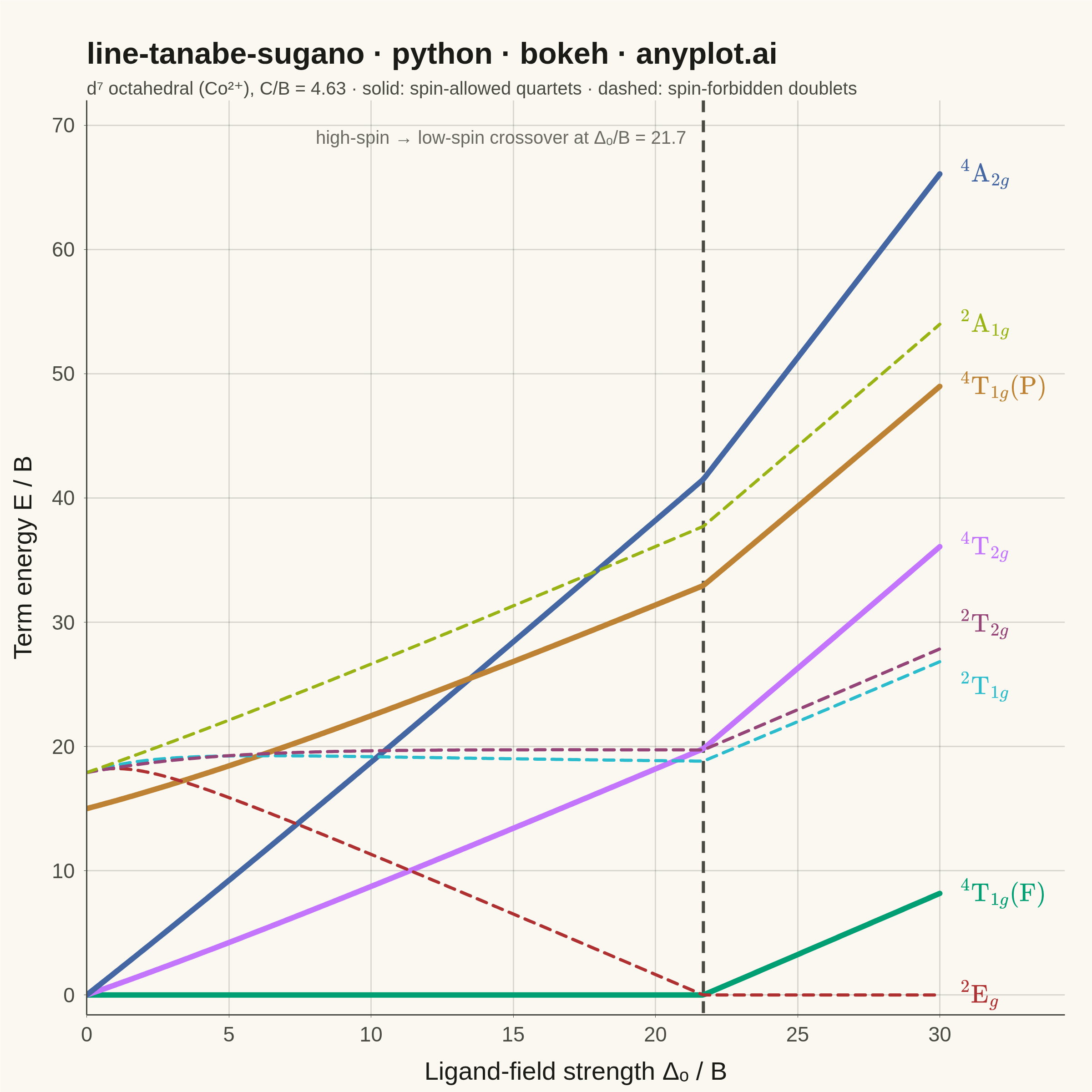
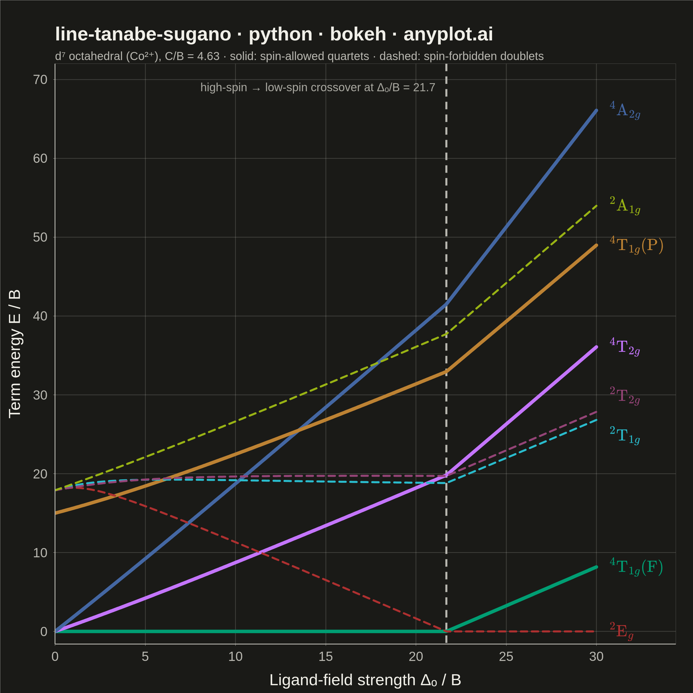
The same plot in 14 other libraries — Python: Altair, lets-plot, Matplotlib, Plotly, plotnine, Pygal, Seaborn; R: ggplot2; Julia: Makie.jl; JavaScript: Chart.js, D3.js, Apache ECharts, Highcharts, MUI X Charts. Compare all 15 side by side: Tanabe-Sugano Diagram for Crystal Field Theory in Python, R, Julia and JavaScript.
A Tanabe-Sugano diagram plots the energies of the electronic term states of a transition-metal ion in an octahedral ligand field as continuous functions of the field strength. The x-axis is the reduced ligand-field strength Δ_o/B (octahedral splitting divided by the Racah parameter B) and the y-axis is the reduced term energy E/B measured from the ground term, which therefore runs along the x-axis itself as a horizontal line at E/B = 0. Each term — labeled with its full symbol including spin multiplicity and Mulliken label — is one curve, and for d⁴–d⁷ a vertical line marks the high-spin/low-spin crossover where the ground term changes and every curve kinks. Chemists read the chart in reverse: matching ratios of observed UV-Vis band energies against the curves yields both Δ_o and B for a real complex.
""" anyplot.ai
line-tanabe-sugano: Tanabe-Sugano Diagram for Crystal Field Theory
Library: bokeh 3.10.0 | Python 3.13.15
Quality: 90/100 | Created: 2026-10-01
"""

import os
import time
from pathlib import Path

import numpy as np
from bokeh.io import output_file, save
from bokeh.models import ColumnDataSource, Label, Span, Title
from bokeh.plotting import figure
from selenium import webdriver
from selenium.webdriver.chrome.options import Options


# Theme tokens (see prompts/default-style-guide.md "Theme-adaptive Chrome")
THEME = os.getenv("ANYPLOT_THEME", "light")
PAGE_BG = "#FAF8F1" if THEME == "light" else "#1A1A17"
INK = "#1A1A17" if THEME == "light" else "#F0EFE8"
INK_SOFT = "#4A4A44" if THEME == "light" else "#B8B7B0"
INK_MUTED = "#6B6A63" if THEME == "light" else "#A8A79F"

# Imprint palette — canonical order, first series is always #009E73
IMPRINT_PALETTE = ["#009E73", "#C475FD", "#4467A3", "#BD8233", "#AE3030", "#2ABCCD", "#954477", "#99B314"]

# Data — d7 (Co2+) in an octahedral field, Racah C/B = 4.633
racah_b = 1.0
racah_c = 4.633 * racah_b
field_strength = np.linspace(0.0, 30.0, 321)  # delta_o / B
dq = field_strength / 10.0  # delta_o = 10 Dq
sqrt2, sqrt3 = np.sqrt(2.0), np.sqrt(3.0)

# Tanabe-Sugano matrices for d7: one symmetry/multiplicity block each, given as
# (diagonal, upper-triangle couplings) in units of B at the chosen C/B.
ts_blocks = {
    "quartet_t1": ([2 * dq - 3 * racah_b, -8 * dq - 12 * racah_b], {(0, 1): 6 * racah_b}),
    "doublet_e": (
        [
            12 * dq - 6 * racah_b + 3 * racah_c,
            2 * dq + 8 * racah_b + 6 * racah_c,
            2 * dq - racah_b + 3 * racah_c,
            -18 * dq - 8 * racah_b + 4 * racah_c,
        ],
        {
            (0, 1): -6 * sqrt2 * racah_b,
            (0, 2): -3 * sqrt2 * racah_b,
            (1, 2): 10 * racah_b,
            (1, 3): sqrt3 * (2 * racah_b + racah_c),
            (2, 3): 2 * sqrt3 * racah_b,
        },
    ),
    "doublet_t1": (
        [
            12 * dq - 6 * racah_b + 3 * racah_c,
            2 * dq + 3 * racah_c,
            2 * dq - 6 * racah_b + 3 * racah_c,
            -8 * dq - 6 * racah_b + 3 * racah_c,
            -8 * dq - 2 * racah_b + 3 * racah_c,
        ],
        {
            (0, 1): -3 * racah_b,
            (0, 2): 3 * racah_b,
            (0, 4): -2 * sqrt3 * racah_b,
            (1, 2): -3 * racah_b,
            (1, 3): 3 * racah_b,
            (1, 4): 3 * sqrt3 * racah_b,
            (2, 3): -3 * racah_b,
            (2, 4): -sqrt3 * racah_b,
            (3, 4): 2 * sqrt3 * racah_b,
        },
    ),
    "doublet_t2": (
        [
            12 * dq + 5 * racah_c,
            2 * dq - 6 * racah_b + 3 * racah_c,
            2 * dq + 4 * racah_b + 3 * racah_c,
            -8 * dq + 6 * racah_b + 5 * racah_c,
            -8 * dq - 2 * racah_b + 3 * racah_c,
        ],
        {
            (0, 1): -3 * sqrt3 * racah_b,
            (0, 2): -5 * sqrt3 * racah_b,
            (0, 3): 4 * racah_b + 2 * racah_c,
            (0, 4): 2 * racah_b,
            (1, 2): 3 * racah_b,
            (1, 3): -3 * sqrt3 * racah_b,
            (1, 4): -3 * sqrt3 * racah_b,
            (2, 3): -sqrt3 * racah_b,
            (2, 4): sqrt3 * racah_b,
            (3, 4): 10 * racah_b,
        },
    ),
}

# Diagonalize every block over the whole field range at once; eigvalsh returns
# ascending levels, so terms of one symmetry avoid each other instead of crossing.
levels = {}
for name, (diagonal, couplings) in ts_blocks.items():
    matrix = np.zeros((field_strength.size, len(diagonal), len(diagonal)))
    for index, element in enumerate(diagonal):
        matrix[:, index, index] = element
    for (row, column), element in couplings.items():
        matrix[:, row, column] = matrix[:, column, row] = element
    levels[name] = np.linalg.eigvalsh(matrix)

# The ground term switches from high-spin 4T1g to low-spin 2Eg at the crossover
ground = np.minimum(levels["quartet_t1"][:, 0], levels["doublet_e"][:, 0])
crossover = np.interp(0.0, levels["quartet_t1"][:, 0] - levels["doublet_e"][:, 0], field_strength)

# Term curves: plain-text key, typeset label, raw energy, label nudge in E/B
terms = (
    ("⁴T₁g(F)", r"$$^{4}\mathrm{T}_{1g}(\mathrm{F})$$", levels["quartet_t1"][:, 0], 0.0),
    ("⁴T₂g", r"$$^{4}\mathrm{T}_{2g}$$", 2 * dq - 15 * racah_b, 0.0),
    ("⁴A₂g", r"$$^{4}\mathrm{A}_{2g}$$", 12 * dq - 15 * racah_b, 0.0),
    ("⁴T₁g(P)", r"$$^{4}\mathrm{T}_{1g}(\mathrm{P})$$", levels["quartet_t1"][:, 1], 0.0),
    ("²Eg", r"$$^{2}\mathrm{E}_{g}$$", levels["doublet_e"][:, 0], 0.0),
    ("²T₁g", r"$$^{2}\mathrm{T}_{1g}$$", levels["doublet_t1"][:, 0], -2.0),
    ("²T₂g", r"$$^{2}\mathrm{T}_{2g}$$", levels["doublet_t2"][:, 0], 2.0),
    ("²A₁g", r"$$^{2}\mathrm{A}_{1g}$$", 2 * dq - 11 * racah_b + 3 * racah_c, 0.0),
)

# Plot — square canvas, the near-square plot area the diagram is read on
p = figure(
    width=2400,
    height=2400,
    title="line-tanabe-sugano · python · bokeh · anyplot.ai",
    x_axis_label="Ligand-field strength Δₒ / B",
    y_axis_label="Term energy E / B",
    x_range=(0.0, 34.4),
    y_range=(-1.6, 72.0),
    toolbar_location=None,
    min_border_bottom=170,
    min_border_left=190,
    min_border_top=220,
    min_border_right=60,
)

for color, (term, typeset, energy, nudge) in zip(IMPRINT_PALETTE, terms, strict=True):
    spin_allowed = term.startswith("⁴")  # same multiplicity as the 4T1g ground term
    source = ColumnDataSource(data={"field": field_strength, "energy": energy - ground})
    p.line(
        x="field",
        y="energy",
        source=source,
        line_color=color,
        line_width=12 if spin_allowed else 7,
        line_dash="solid" if spin_allowed else [22, 16],
        line_cap="round",
    )
    p.add_layout(
        Label(
            x=field_strength[-1] + 0.7,
            y=energy[-1] - ground[-1] + nudge,
            text=typeset,
            text_color=color,
            text_font_size="34pt",
            text_baseline="middle",
        )
    )

# Crossover: every curve kinks here because the reference ground term changes
p.add_layout(
    Span(
        location=crossover, dimension="height", line_color=INK_SOFT, line_dash=[26, 18], line_width=7, level="underlay"
    )
)
p.add_layout(
    Label(
        x=crossover - 0.6,
        y=69.0,
        text=f"high-spin → low-spin crossover at Δₒ/B = {crossover:.1f}",
        text_color=INK_MUTED,
        text_font_size="30pt",
        text_align="right",
        text_baseline="middle",
    )
)

# Style
p.add_layout(
    Title(
        text="d⁷ octahedral (Co²⁺), C/B = 4.63 · solid: spin-allowed quartets · dashed: spin-forbidden doublets",
        text_color=INK_SOFT,
        text_font_size="30pt",
        text_font_style="normal",
    ),
    "above",
)
p.background_fill_color = PAGE_BG
p.border_fill_color = PAGE_BG
p.outline_line_color = None
p.title.text_color = INK
p.title.text_font_size = "50pt"
p.title.standoff = 26
p.axis.axis_label_text_color = INK
p.axis.axis_label_text_font_size = "42pt"
p.axis.axis_label_text_font_style = "normal"
p.axis.axis_label_standoff = 30
p.axis.major_label_text_color = INK_SOFT
p.axis.major_label_text_font_size = "34pt"
p.axis.major_label_standoff = 20
p.axis.axis_line_color = INK_SOFT
p.axis.axis_line_width = 3
p.axis.major_tick_line_color = INK_SOFT
p.axis.minor_tick_line_color = None
p.grid.grid_line_color = INK
p.grid.grid_line_alpha = 0.15
p.grid.grid_line_width = 3

# Save — interactive HTML plus a headless-Chrome screenshot for the gallery PNG
output_file(f"plot-{THEME}.html")
save(p)

W, H = 2400, 2400
opts = Options()
for arg in (
    "--headless=new",
    "--no-sandbox",
    "--disable-dev-shm-usage",
    "--disable-gpu",
    f"--window-size={W},{H}",
    "--hide-scrollbars",
):
    opts.add_argument(arg)
driver = webdriver.Chrome(options=opts)
driver.set_window_size(W, H)
driver.get(f"file://{Path(f'plot-{THEME}.html').resolve()}")
driver.execute_cdp_cmd(
    "Emulation.setDeviceMetricsOverride", {"width": W, "height": H, "deviceScaleFactor": 1, "mobile": False}
)
time.sleep(6)  # let bokeh render the canvas and MathJax typeset the term labels
driver.save_screenshot(f"plot-{THEME}.png")
driver.quit()
Runnable source as JSON, for any HTTP client: https://api.anyplot.ai/specs/line-tanabe-sugano/bokeh/code. Any spec id and library id listed in llms-full.txt fit the same URL shape; every URL below is complete and callable.
{
  "spec_id": "line-tanabe-sugano",
  "language": "python",
  "library": "bokeh",
  "page": "https://anyplot.ai/line-tanabe-sugano/python/bokeh",
  "hub": "https://anyplot.ai/line-tanabe-sugano",
  "code_json": "https://api.anyplot.ai/specs/line-tanabe-sugano/bokeh/code",
  "spec_json": "https://api.anyplot.ai/specs/line-tanabe-sugano",
  "render_light_png": "https://storage.googleapis.com/anyplot-images/plots/line-tanabe-sugano/python/bokeh/plot-light.png",
  "render_dark_png": "https://storage.googleapis.com/anyplot-images/plots/line-tanabe-sugano/python/bokeh/plot-dark.png",
  "interactive_light_html": "https://storage.googleapis.com/anyplot-images/plots/line-tanabe-sugano/python/bokeh/plot-light.html",
  "interactive_dark_html": "https://storage.googleapis.com/anyplot-images/plots/line-tanabe-sugano/python/bokeh/plot-dark.html",
  "quality_score": 90.0,
  "license": "MIT",
  "guide": "https://anyplot.ai/llms.txt"
}
Part of Tanabe-Sugano Diagram for Crystal Field Theory on anyplot.ai.