The same plot in 14 other libraries — Python: Altair, Bokeh, lets-plot, Matplotlib, Plotly, plotnine, Pygal; R: ggplot2; Julia: Makie.jl; JavaScript: Chart.js, D3.js, Apache ECharts, Highcharts, MUI X Charts. Compare all 15 side by side: Tanabe-Sugano Diagram for Crystal Field Theory in Python, R, Julia and JavaScript.
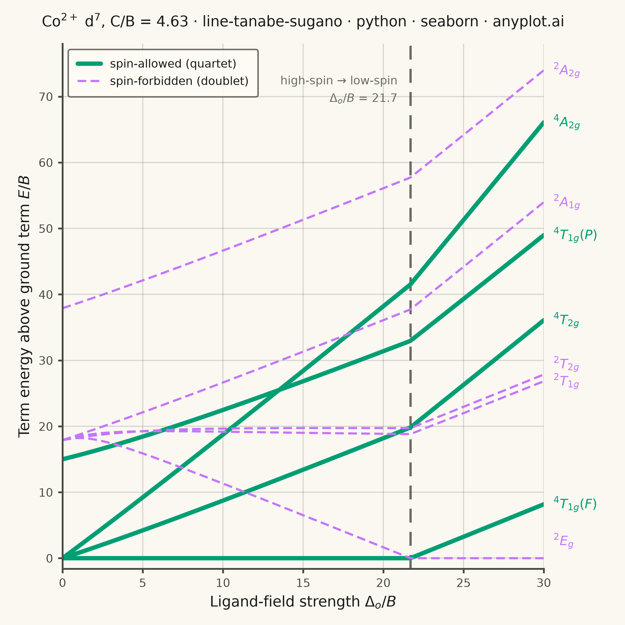
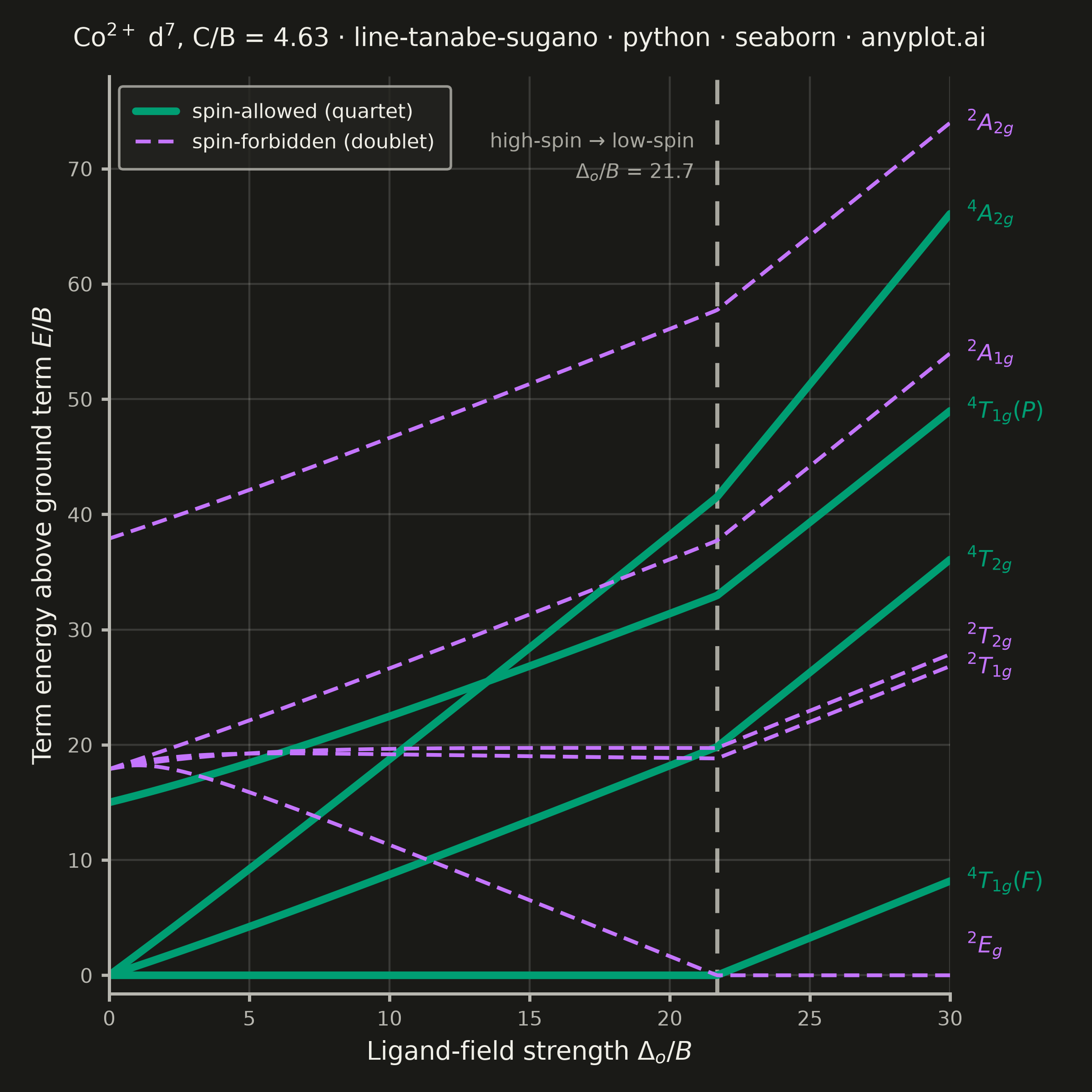
A Tanabe-Sugano diagram plots the energies of the electronic term states of a transition-metal ion in an octahedral ligand field as continuous functions of the field strength. The x-axis is the reduced ligand-field strength Δ_o/B (octahedral splitting divided by the Racah parameter B) and the y-axis is the reduced term energy E/B measured from the ground term, which therefore runs along the x-axis itself as a horizontal line at E/B = 0. Each term — labeled with its full symbol including spin multiplicity and Mulliken label — is one curve, and for d⁴–d⁷ a vertical line marks the high-spin/low-spin crossover where the ground term changes and every curve kinks. Chemists read the chart in reverse: matching ratios of observed UV-Vis band energies against the curves yields both Δ_o and B for a real complex.
""" anyplot.ai
line-tanabe-sugano: Tanabe-Sugano Diagram for Crystal Field Theory
Library: seaborn 0.13.2 | Python 3.13.15
Quality: 90/100 | Created: 2026-10-01
"""

import os

import matplotlib.pyplot as plt
import numpy as np
import pandas as pd
import seaborn as sns


# Theme tokens (see prompts/default-style-guide.md "Theme-adaptive Chrome")
THEME = os.getenv("ANYPLOT_THEME", "light")
PAGE_BG = "#FAF8F1" if THEME == "light" else "#1A1A17"
ELEVATED_BG = "#FFFDF6" if THEME == "light" else "#242420"
INK = "#1A1A17" if THEME == "light" else "#F0EFE8"
INK_SOFT = "#4A4A44" if THEME == "light" else "#B8B7B0"
INK_MUTED = "#6B6A63" if THEME == "light" else "#A8A79F"

# Imprint palette — spin-allowed is position 1 (brand green), spin-forbidden position 2
ALLOWED = "spin-allowed (quartet)"
FORBIDDEN = "spin-forbidden (doublet)"
SPIN_COLORS = {ALLOWED: "#009E73", FORBIDDEN: "#C475FD"}

# Data — d7 (Co2+) in an octahedral field: the Tanabe-Sugano matrices in the
# strong-field basis, written in units of B with Dq/B on the diagonal
# (Tanabe & Sugano, J. Phys. Soc. Jpn. 9, 753 (1954); C/B is their d7 value).
C_OVER_B = 4.633
delta_over_b = np.linspace(0, 30, 301)
dq = delta_over_b / 10  # Delta_o = 10 Dq
sqrt2, sqrt3 = np.sqrt(2), np.sqrt(3)

ts_blocks = {
    "4T1": ([2 * dq - 3, -8 * dq - 12], {(0, 1): 6}),
    "4T2": ([2 * dq - 15], {}),
    "4A2": ([12 * dq - 15], {}),
    "2A1": ([2 * dq - 11 + 3 * C_OVER_B], {}),
    "2A2": ([2 * dq + 9 + 3 * C_OVER_B], {}),
    "2E": (
        [12 * dq - 6 + 3 * C_OVER_B, 2 * dq + 8 + 6 * C_OVER_B, 2 * dq - 1 + 3 * C_OVER_B, -18 * dq - 8 + 4 * C_OVER_B],
        {(0, 1): -6 * sqrt2, (0, 2): -3 * sqrt2, (1, 2): 10, (1, 3): sqrt3 * (2 + C_OVER_B), (2, 3): 2 * sqrt3},
    ),
    "2T1": (
        [
            12 * dq - 6 + 3 * C_OVER_B,
            2 * dq + 3 * C_OVER_B,
            2 * dq - 6 + 3 * C_OVER_B,
            -8 * dq - 6 + 3 * C_OVER_B,
            -8 * dq - 2 + 3 * C_OVER_B,
        ],
        {
            (0, 1): -3,
            (0, 2): 3,
            (0, 4): -2 * sqrt3,
            (1, 2): -3,
            (1, 3): 3,
            (1, 4): 3 * sqrt3,
            (2, 3): -3,
            (2, 4): -sqrt3,
            (3, 4): 2 * sqrt3,
        },
    ),
    "2T2": (
        [
            12 * dq + 5 * C_OVER_B,
            2 * dq - 6 + 3 * C_OVER_B,
            2 * dq + 4 + 3 * C_OVER_B,
            -8 * dq + 6 + 5 * C_OVER_B,
            -8 * dq - 2 + 3 * C_OVER_B,
        ],
        {
            (0, 1): -3 * sqrt3,
            (0, 2): -5 * sqrt3,
            (0, 3): 4 + 2 * C_OVER_B,
            (0, 4): 2,
            (1, 2): 3,
            (1, 3): -3 * sqrt3,
            (1, 4): -3 * sqrt3,
            (2, 3): -sqrt3,
            (2, 4): sqrt3,
            (3, 4): 10,
        },
    ),
}

# Diagonalize every symmetry block at each field strength (roots come out ascending,
# so terms of the same symmetry and spin only ever approach, never cross)
block_roots = {}
for block, (diagonal, off_diagonal) in ts_blocks.items():
    size = len(diagonal)
    matrices = np.zeros((delta_over_b.size, size, size))
    for i, element in enumerate(diagonal):
        matrices[:, i, i] = element
    for (i, j), element in off_diagonal.items():
        matrices[:, i, j] = matrices[:, j, i] = element
    block_roots[block] = np.linalg.eigvalsh(matrices)

# Term symbol, its symmetry block, which root of that block, spin class
terms = [
    (r"$^{4}T_{1g}(F)$", "4T1", 0, ALLOWED),
    (r"$^{4}T_{2g}$", "4T2", 0, ALLOWED),
    (r"$^{4}A_{2g}$", "4A2", 0, ALLOWED),
    (r"$^{4}T_{1g}(P)$", "4T1", 1, ALLOWED),
    (r"$^{2}E_{g}$", "2E", 0, FORBIDDEN),
    (r"$^{2}T_{1g}$", "2T1", 0, FORBIDDEN),
    (r"$^{2}T_{2g}$", "2T2", 0, FORBIDDEN),
    (r"$^{2}A_{1g}$", "2A1", 0, FORBIDDEN),
    (r"$^{2}A_{2g}$", "2A2", 0, FORBIDDEN),
]

# Energies are measured from the ground term, which switches from the high-spin
# 4T1g to the low-spin 2Eg at the crossover and kinks every curve there
ground_energy = np.min([block_roots[block][:, root] for _, block, root, _ in terms], axis=0)
curves = pd.concat(
    [
        pd.DataFrame(
            {
                "delta_over_b": delta_over_b,
                "energy_over_b": block_roots[block][:, root] - ground_energy,
                "term": term,
                "spin_class": spin_class,
            }
        )
        for term, block, root, spin_class in terms
    ],
    ignore_index=True,
)
crossover = np.interp(0.0, block_roots["4T1"][:, 0] - block_roots["2E"][:, 0], delta_over_b)

# Plot
sns.set_theme(
    style="ticks",
    rc={
        "figure.facecolor": PAGE_BG,
        "axes.facecolor": PAGE_BG,
        "axes.edgecolor": INK_SOFT,
        "axes.labelcolor": INK,
        "text.color": INK,
        "xtick.color": INK_SOFT,
        "ytick.color": INK_SOFT,
        "grid.color": INK,
        "grid.alpha": 0.15,
        "legend.facecolor": ELEVATED_BG,
        "legend.edgecolor": INK_SOFT,
    },
)
fig, ax = plt.subplots(figsize=(6, 6), dpi=400)
sns.lineplot(
    data=curves,
    x="delta_over_b",
    y="energy_over_b",
    units="term",
    estimator=None,
    hue="spin_class",
    style="spin_class",
    size="spin_class",
    hue_order=[ALLOWED, FORBIDDEN],
    palette=SPIN_COLORS,
    dashes={ALLOWED: "", FORBIDDEN: (4, 2)},
    sizes={ALLOWED: 3.0, FORBIDDEN: 1.5},
    ax=ax,
)

# High-spin / low-spin crossover
ax.axvline(crossover, color=INK_MUTED, linestyle=(0, (6, 4)), linewidth=1.6, zorder=0)
ax.text(
    crossover - 0.8,
    71,
    f"high-spin → low-spin\n$\\Delta_o/B$ = {crossover:.1f}",
    ha="right",
    va="center",
    fontsize=8,
    color=INK_MUTED,
    linespacing=1.5,
)

# Term labels at the right edge, nudged apart where curves converge
label_y = 0.0
for end_energy, term, spin_class in sorted(
    (float(block_roots[block][-1, root] - ground_energy[-1]), term, spin_class)
    for term, block, root, spin_class in terms
):
    label_y = max(end_energy, label_y + 2.6)
    ax.text(
        delta_over_b[-1] + 0.6, label_y, term, va="center", fontsize=9, color=SPIN_COLORS[spin_class], clip_on=False
    )

# Style
ax.set_title(
    "Co$^{2+}$ d$^7$, C/B = 4.63 · line-tanabe-sugano · python · seaborn · anyplot.ai",
    fontsize=10,
    fontweight="medium",
    color=INK,
    pad=12,
)
ax.set_xlabel("Ligand-field strength $\\Delta_o/B$", fontsize=10)
ax.set_ylabel("Term energy above ground term $E/B$", fontsize=10)
ax.set_xlim(0, 30)
ax.set_ylim(-1.6, 78)
ax.set_xticks(np.arange(0, 31, 5))
ax.set_yticks(np.arange(0, 78, 10))
ax.tick_params(axis="both", labelsize=8, length=3)
ax.grid(True, alpha=0.15, linewidth=0.8)
ax.legend(*ax.get_legend_handles_labels(), title=None, fontsize=8, loc="upper left", borderpad=0.8)
sns.despine(ax=ax)
fig.subplots_adjust(left=0.1, right=0.87, top=0.93, bottom=0.09)

# Save
plt.savefig(f"plot-{THEME}.png", dpi=400, facecolor=PAGE_BG)
Runnable source as JSON, for any HTTP client: https://api.anyplot.ai/specs/line-tanabe-sugano/seaborn/code. Any spec id and library id listed in llms-full.txt fit the same URL shape; every URL below is complete and callable.
{
  "spec_id": "line-tanabe-sugano",
  "language": "python",
  "library": "seaborn",
  "page": "https://anyplot.ai/line-tanabe-sugano/python/seaborn",
  "hub": "https://anyplot.ai/line-tanabe-sugano",
  "code_json": "https://api.anyplot.ai/specs/line-tanabe-sugano/seaborn/code",
  "spec_json": "https://api.anyplot.ai/specs/line-tanabe-sugano",
  "render_light_png": "https://storage.googleapis.com/anyplot-images/plots/line-tanabe-sugano/python/seaborn/plot-light.png",
  "render_dark_png": "https://storage.googleapis.com/anyplot-images/plots/line-tanabe-sugano/python/seaborn/plot-dark.png",
  "quality_score": 90.0,
  "license": "MIT",
  "guide": "https://anyplot.ai/llms.txt"
}
Part of Tanabe-Sugano Diagram for Crystal Field Theory on anyplot.ai.