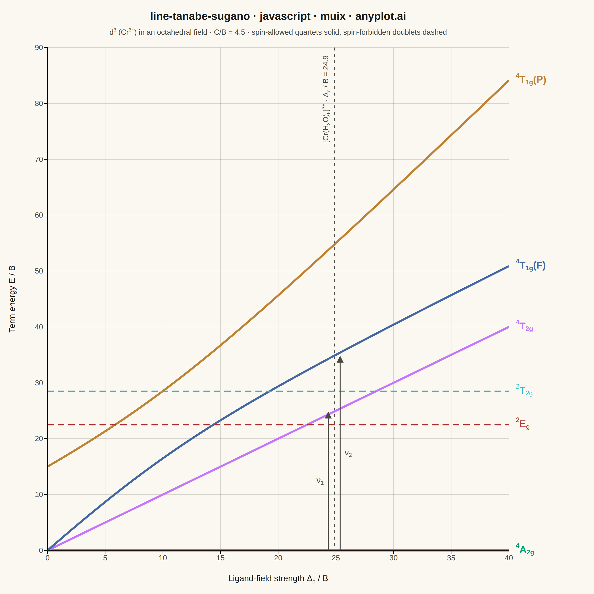
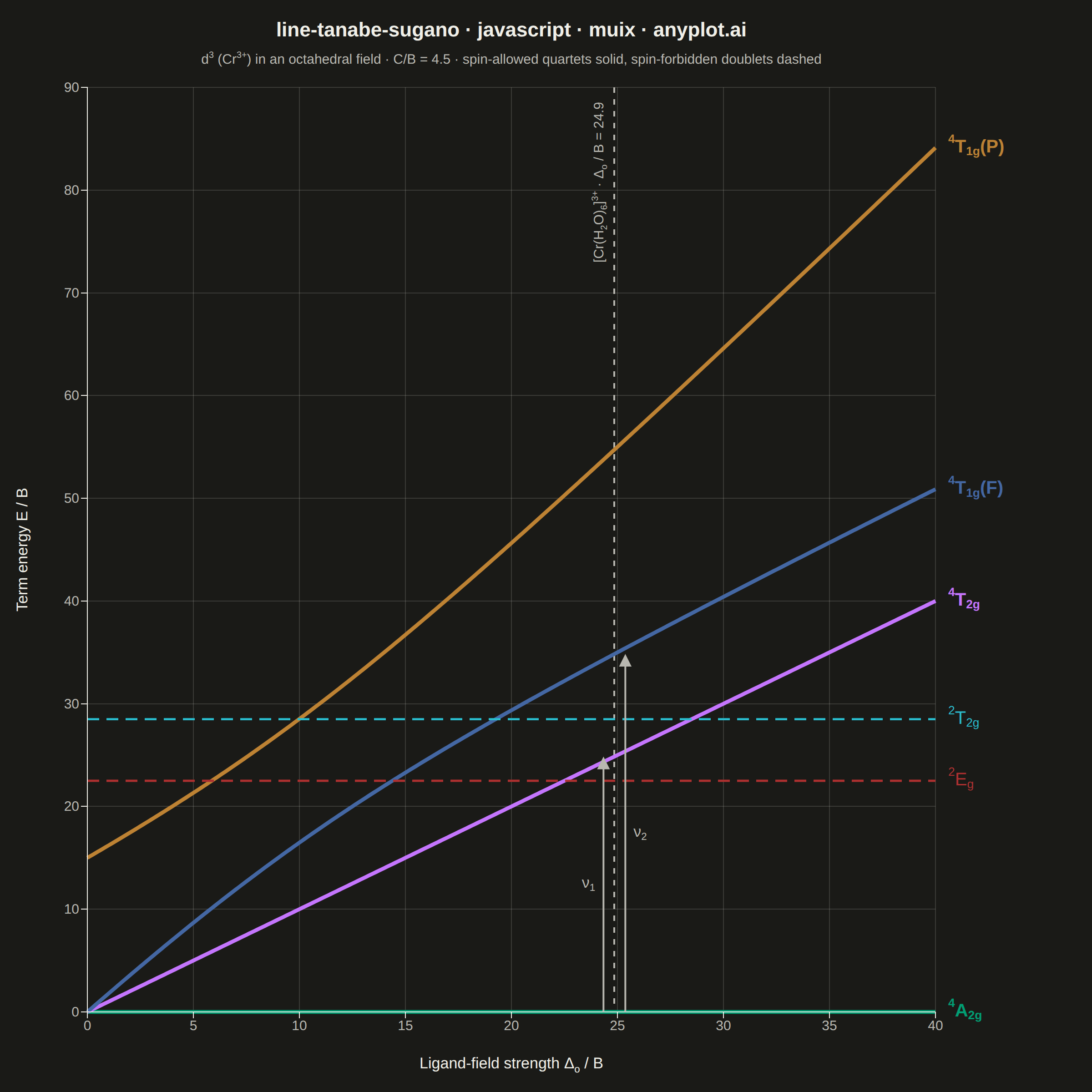
The same plot in 14 other libraries — JavaScript: Chart.js, D3.js, Apache ECharts, Highcharts; Python: Altair, Bokeh, lets-plot, Matplotlib, Plotly, plotnine, Pygal, Seaborn; R: ggplot2; Julia: Makie.jl. Compare all 15 side by side: Tanabe-Sugano Diagram for Crystal Field Theory in Python, R, Julia and JavaScript.
A Tanabe-Sugano diagram plots the energies of the electronic term states of a transition-metal ion in an octahedral ligand field as continuous functions of the field strength. The x-axis is the reduced ligand-field strength Δ_o/B (octahedral splitting divided by the Racah parameter B) and the y-axis is the reduced term energy E/B measured from the ground term, which therefore runs along the x-axis itself as a horizontal line at E/B = 0. Each term — labeled with its full symbol including spin multiplicity and Mulliken label — is one curve, and for d⁴–d⁷ a vertical line marks the high-spin/low-spin crossover where the ground term changes and every curve kinks. Chemists read the chart in reverse: matching ratios of observed UV-Vis band energies against the curves yields both Δ_o and B for a real complex.
// anyplot.ai
// line-tanabe-sugano: Tanabe-Sugano Diagram for Crystal Field Theory
// Library: muix 7.29.1 | JavaScript 22.23.3
// Quality: 90/100 | Created: 2026-10-01
//# anyplot-orientation: square
// anyplot.ai
// line-tanabe-sugano: Tanabe-Sugano Diagram for Crystal Field Theory
// Library: MUI X Charts | React | Node 22
// License: @mui/x-charts — MIT (community). Pro/Premium are out of scope.
// Quality: pending | Created: 2026-10-01
import { ChartContainer } from "@mui/x-charts/ChartContainer";
import { LinePlot } from "@mui/x-charts/LineChart";
import { ChartsXAxis } from "@mui/x-charts/ChartsXAxis";
import { ChartsYAxis } from "@mui/x-charts/ChartsYAxis";
import { ChartsGrid } from "@mui/x-charts/ChartsGrid";
import { ChartsReferenceLine } from "@mui/x-charts/ChartsReferenceLine";
import { ChartsTooltip } from "@mui/x-charts/ChartsTooltip";
import { useDrawingArea, useXScale, useYScale } from "@mui/x-charts/hooks";

const t = window.ANYPLOT_TOKENS;
const { width: WIDTH, height: HEIGHT } = window.ANYPLOT_SIZE;
const MARGIN = { top: 96, right: 172, bottom: 88, left: 96 };

// Data — d³ (Cr³⁺) in an octahedral field at C/B = 4.5, energies in units of B
const C_OVER_B = 4.5;
const FIELD_MAX = 40;
const ENERGY_MAX = 90;
const fieldStrengths = Array.from({ length: 321 }, (_, i) => (i * FIELD_MAX) / 320);

// ⁴T₁g is the only Tanabe-Sugano block of d³ bigger than 1×1. In the weak-field
// basis (⁴F and ⁴P parents), relative to the ⁴A₂g ground term, with d = Δo/B:
//     [ 1.8d         0.4d  ]
//     [ 0.4d    15 + 1.2d  ]
// Both ⁴T₁g curves are eigenvalues of that symmetric matrix, so the avoided
// crossing is the 12B gap the matrix itself keeps at d = 9 — never a spline.
const t1gEigenvalues = (d) => {
  const [t1gF, t1gP, mixing] = [1.8 * d, 15 + 1.2 * d, 0.4 * d];
  const centre = (t1gF + t1gP) / 2;
  const splitting = Math.hypot((t1gF - t1gP) / 2, mixing);
  return [centre - splitting, centre + splitting];
};

// Term symbols as [kind, text] runs, typeset below into true super/subscripts.
// The spin-forbidden doublets both belong to the same t₂g³ configuration as the
// ⁴A₂g ground term, so their Racah energies carry no first-order Dq term at all
// and the curves run horizontally — 9B + 3C and 15B + 3C.
const TERMS = [
  { id: "a2g", key: "⁴A₂g", runs: [["sup", "4"], ["base", "A"], ["sub", "2g"]],
    spinAllowed: true, energy: () => 0 },
  { id: "t2g", key: "⁴T₂g", runs: [["sup", "4"], ["base", "T"], ["sub", "2g"]],
    spinAllowed: true, energy: (d) => d },
  { id: "t1gF", key: "⁴T₁g(F)", runs: [["sup", "4"], ["base", "T"], ["sub", "1g"], ["base", "(F)"]],
    spinAllowed: true, energy: (d) => t1gEigenvalues(d)[0] },
  { id: "t1gP", key: "⁴T₁g(P)", runs: [["sup", "4"], ["base", "T"], ["sub", "1g"], ["base", "(P)"]],
    spinAllowed: true, energy: (d) => t1gEigenvalues(d)[1] },
  { id: "eg", key: "²Eg", runs: [["sup", "2"], ["base", "E"], ["sub", "g"]],
    spinAllowed: false, energy: () => 9 + 3 * C_OVER_B },
  { id: "t2gDoublet", key: "²T₂g", runs: [["sup", "2"], ["base", "T"], ["sub", "2g"]],
    spinAllowed: false, energy: () => 15 + 3 * C_OVER_B },
];

// [Cr(H₂O)₆]³⁺: Δo = 17 400 cm⁻¹ against B = 700 cm⁻¹ — where a chemist reads
// the diagram off after matching two observed UV-Vis bands.
const EXAMPLE_FIELD = 17400 / 700;

// Typography — the library's own markup is SVG tspans, so multiplicities become
// real superscripts and the numeral plus the g a real subscript.
const SHIFT = { base: 0, sup: -0.42, sub: 0.26 };
const typeset = (runs, size) => {
  let offset = 0;
  return runs.map(([kind, text], i) => {
    const dy = (SHIFT[kind] - offset) * size;
    offset = SHIFT[kind];
    return (
      <tspan key={i} dy={dy} fontSize={kind === "base" ? size : size * 0.66}>
        {text}
      </tspan>
    );
  });
};

// Curve labels sit just outside the right edge at each term's final energy, with
// a greedy vertical declutter so converging labels stay readable (the curves
// themselves never move off their computed energies).
function TermLabels() {
  const { left, width } = useDrawingArea();
  const yScale = useYScale();
  let lowest = -Infinity;
  return (
    <g>
      {TERMS.map((term, i) => ({ term, color: t.palette[i], y: yScale(term.energy(FIELD_MAX)) }))
        .sort((a, b) => a.y - b.y)
        .map(({ term, color, y }) => {
          const placed = Math.max(y, lowest + 32);
          lowest = placed;
          return (
            <text
              key={term.id}
              x={left + width + 14}
              y={placed}
              fill={color}
              fontSize={20}
              fontWeight={term.spinAllowed ? 600 : 500}
              dominantBaseline="middle"
            >
              {typeset(term.runs, 20)}
            </text>
          );
        })}
    </g>
  );
}

// The marker the Notes offer as optional: a vertical line at the Δo/B a chemist
// reads off for [Cr(H₂O)₆]³⁺, with its two observed d–d bands as arrows running
// from the ground term up to the terms they reach.
function ExampleComplex() {
  const xScale = useXScale();
  const yScale = useYScale();
  const x = xScale(EXAMPLE_FIELD);
  const bands = [
    { id: "nu1", runs: [["base", "ν"], ["sub", "1"]], term: TERMS[1], dx: -12 },
    { id: "nu2", runs: [["base", "ν"], ["sub", "2"]], term: TERMS[2], dx: 12 },
  ];
  return (
    <g>
      <defs>
        <marker id="band-arrow" markerUnits="userSpaceOnUse" markerWidth={14} markerHeight={14}
                refX={7} refY={7} orient="auto">
          <path d="M0,0 L14,7 L0,14 z" fill={t.inkSoft} />
        </marker>
      </defs>
      {bands.map(({ id, runs, term, dx }) => (
        <g key={id}>
          <line
            x1={x + dx} y1={yScale(0)} x2={x + dx} y2={yScale(term.energy(EXAMPLE_FIELD)) + 7}
            stroke={t.inkSoft} strokeWidth={2} markerEnd="url(#band-arrow)"
          />
          <text
            x={x + dx + Math.sign(dx) * 9} y={(yScale(0) + yScale(term.energy(EXAMPLE_FIELD))) / 2}
            fill={t.inkSoft} fontSize={17} textAnchor={dx < 0 ? "end" : "start"} dominantBaseline="middle"
          >
            {typeset(runs, 17)}
          </text>
        </g>
      ))}
      <text x={0} y={0} fill={t.inkSoft} fontSize={15} textAnchor="end"
            transform={`translate(${x - 12} ${yScale(ENERGY_MAX) + 16}) rotate(-90)`}>
        {typeset([["base", "[Cr(H"], ["sub", "2"], ["base", "O)"], ["sub", "6"], ["base", "]"], ["sup", "3+"], ["base", " · Δ"], ["sub", "o"], ["base", " / B = 24.9"]], 15)}
      </text>
    </g>
  );
}

// Chart
export default function Chart() {
  return (
    <ChartContainer
      width={WIDTH}
      height={HEIGHT}
      margin={MARGIN}
      colors={t.palette}
      series={TERMS.map((term) => ({
        type: "line",
        id: term.id,
        label: term.key,
        showMark: false,
        curve: "linear",
        data: fieldStrengths.map(term.energy),
      }))}
      xAxis={[{ id: "field", data: fieldStrengths, scaleType: "linear", min: 0, max: FIELD_MAX, tickNumber: 9 }]}
      yAxis={[{ id: "energy", min: 0, max: ENERGY_MAX, tickNumber: 9 }]}
      sx={Object.fromEntries(
        TERMS.map((term) => [
          `& .MuiLineElement-series-${term.id}`,
          term.spinAllowed
            ? { strokeWidth: 4.2 }
            : { strokeWidth: 2.4, strokeDasharray: "13 8" },
        ]),
      )}
    >
      <ChartsGrid vertical horizontal />
      <ChartsReferenceLine
        x={EXAMPLE_FIELD}
        axisId="field"
        lineStyle={{ stroke: t.inkSoft, strokeWidth: 2, strokeDasharray: "6 7" }}
      />
      <LinePlot skipAnimation />
      <ChartsXAxis axisId="field" tickLabelStyle={{ fontSize: 15, fill: t.inkSoft }} tickSize={7} />
      <ChartsYAxis axisId="energy" tickLabelStyle={{ fontSize: 15, fill: t.inkSoft }} tickSize={7} />
      <ExampleComplex />
      <TermLabels />
      <ChartsTooltip trigger="axis" />

      {/* Title, subtitle and axis titles — SVG text so every term symbol and
          formula keeps its super- and subscripts. */}
      <text x={MARGIN.left + (WIDTH - MARGIN.left - MARGIN.right) / 2} y={40} fill={t.ink}
            fontSize={22} fontWeight={600} textAnchor="middle">
        line-tanabe-sugano · javascript · muix · anyplot.ai
      </text>
      <text x={MARGIN.left + (WIDTH - MARGIN.left - MARGIN.right) / 2} y={70} fill={t.inkSoft}
            fontSize={15} textAnchor="middle">
        {typeset([["base", "d"], ["sup", "3"], ["base", " (Cr"], ["sup", "3+"],
          ["base", `) in an octahedral field · C/B = ${C_OVER_B} · spin-allowed quartets solid, spin-forbidden doublets dashed`]], 15)}
      </text>
      <text x={MARGIN.left + (WIDTH - MARGIN.left - MARGIN.right) / 2} y={HEIGHT - 26} fill={t.ink}
            fontSize={17} textAnchor="middle">
        {typeset([["base", "Ligand-field strength Δ"], ["sub", "o"], ["base", " / B"]], 17)}
      </text>
      <text x={30} y={MARGIN.top + (HEIGHT - MARGIN.top - MARGIN.bottom) / 2} fill={t.ink}
            fontSize={17} textAnchor="middle"
            transform={`rotate(-90 30 ${MARGIN.top + (HEIGHT - MARGIN.top - MARGIN.bottom) / 2})`}>
        Term energy E / B
      </text>
    </ChartContainer>
  );
}
Runnable source as JSON, for any HTTP client: https://api.anyplot.ai/specs/line-tanabe-sugano/muix/code. Any spec id and library id listed in llms-full.txt fit the same URL shape; every URL below is complete and callable.
{
  "spec_id": "line-tanabe-sugano",
  "language": "javascript",
  "library": "muix",
  "page": "https://anyplot.ai/line-tanabe-sugano/javascript/muix",
  "hub": "https://anyplot.ai/line-tanabe-sugano",
  "code_json": "https://api.anyplot.ai/specs/line-tanabe-sugano/muix/code",
  "spec_json": "https://api.anyplot.ai/specs/line-tanabe-sugano",
  "render_light_png": "https://storage.googleapis.com/anyplot-images/plots/line-tanabe-sugano/javascript/muix/plot-light.png",
  "render_dark_png": "https://storage.googleapis.com/anyplot-images/plots/line-tanabe-sugano/javascript/muix/plot-dark.png",
  "interactive_light_html": "https://storage.googleapis.com/anyplot-images/plots/line-tanabe-sugano/javascript/muix/plot-light.html",
  "interactive_dark_html": "https://storage.googleapis.com/anyplot-images/plots/line-tanabe-sugano/javascript/muix/plot-dark.html",
  "quality_score": 90.0,
  "license": "MIT",
  "guide": "https://anyplot.ai/llms.txt"
}
Part of Tanabe-Sugano Diagram for Crystal Field Theory on anyplot.ai.