The same plot in 14 other libraries — Python: Altair, Bokeh, lets-plot, Matplotlib, Plotly, plotnine, Pygal, Seaborn; Julia: Makie.jl; JavaScript: Chart.js, D3.js, Apache ECharts, Highcharts, MUI X Charts. Compare all 15 side by side: Tanabe-Sugano Diagram for Crystal Field Theory in Python, R, Julia and JavaScript.
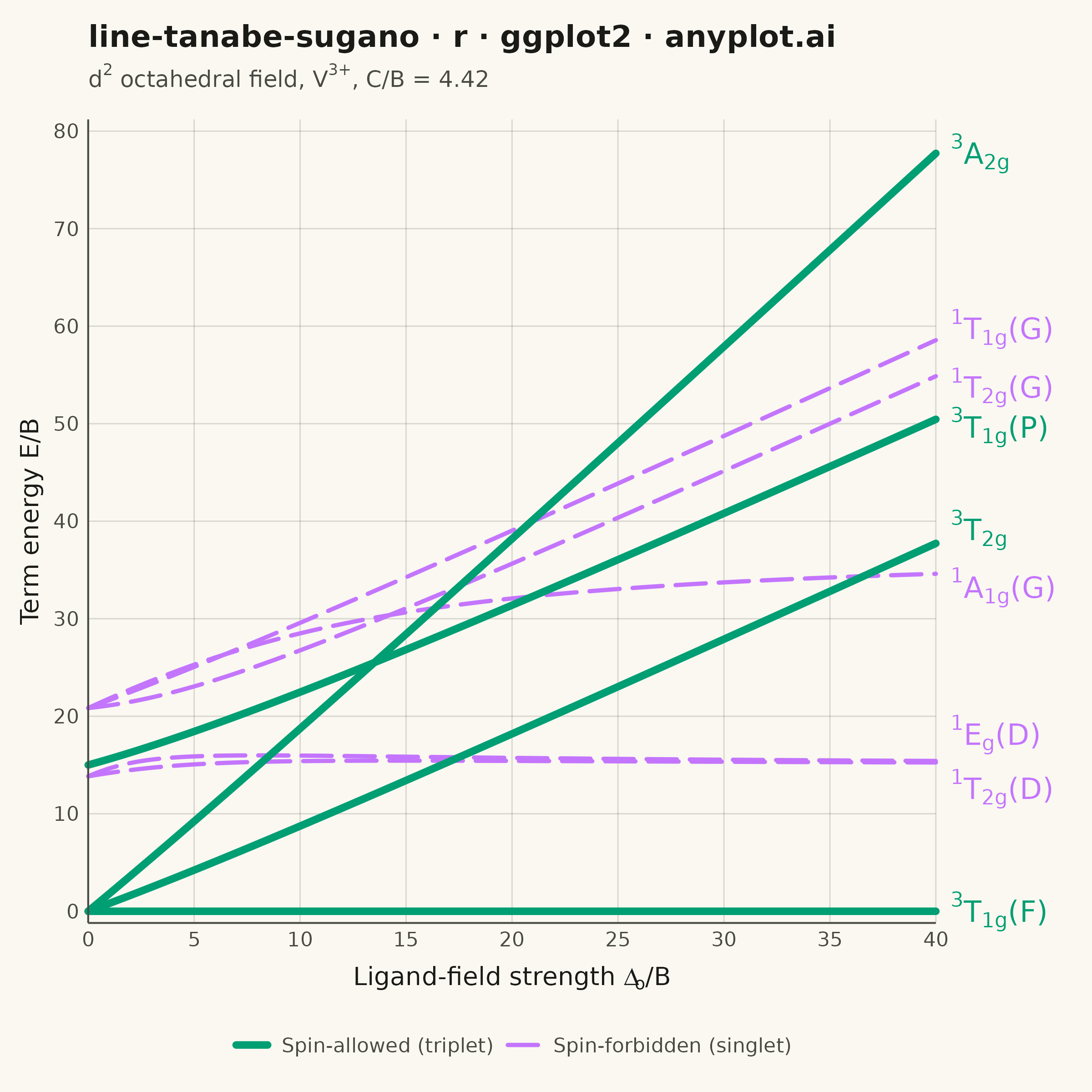
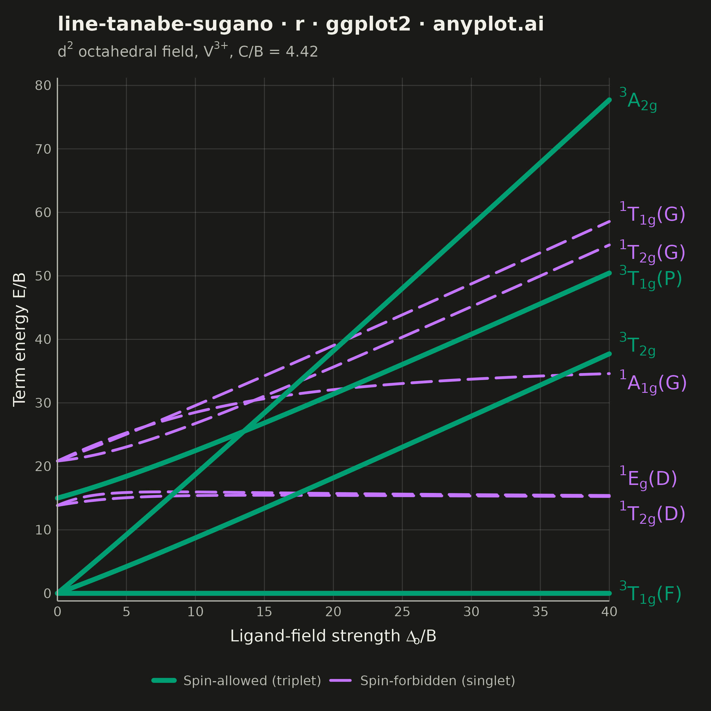
A Tanabe-Sugano diagram plots the energies of the electronic term states of a transition-metal ion in an octahedral ligand field as continuous functions of the field strength. The x-axis is the reduced ligand-field strength Δ_o/B (octahedral splitting divided by the Racah parameter B) and the y-axis is the reduced term energy E/B measured from the ground term, which therefore runs along the x-axis itself as a horizontal line at E/B = 0. Each term — labeled with its full symbol including spin multiplicity and Mulliken label — is one curve, and for d⁴–d⁷ a vertical line marks the high-spin/low-spin crossover where the ground term changes and every curve kinks. Chemists read the chart in reverse: matching ratios of observed UV-Vis band energies against the curves yields both Δ_o and B for a real complex.
#' anyplot.ai
#' line-tanabe-sugano: Tanabe-Sugano Diagram for Crystal Field Theory
#' Library: ggplot2 3.5.1 | R 4.4.1
#' Quality: 91/100 | Created: 2026-10-01

library(ggplot2)
library(dplyr)
library(tidyr)
library(scales)
library(ragg)

# --- Theme tokens -----------------------------------------------------------
THEME    <- Sys.getenv("ANYPLOT_THEME", "light")
PAGE_BG  <- if (THEME == "light") "#FAF8F1" else "#1A1A17"
INK      <- if (THEME == "light") "#1A1A17" else "#F0EFE8"
INK_SOFT <- if (THEME == "light") "#4A4A44" else "#B8B7B0"

# Imprint palette: position 1 (brand green) carries the spin-allowed terms,
# position 2 (lavender) the spin-forbidden ones.
SPIN_ALLOWED   <- "#009E73"
SPIN_FORBIDDEN <- "#C475FD"
ALLOWED_LABEL   <- "Spin-allowed (triplet)"
FORBIDDEN_LABEL <- "Spin-forbidden (singlet)"

# --- Data: octahedral d2 term energies (V3+, C/B = 4.42) --------------------
# Energies are in units of the Racah parameter B, the centroid A dropped. A
# term symbol that occurs in two strong-field configurations gets a 2x2
# secular block whose off-diagonal element mixes them; both roots of the block
# are real term energies, and because the mixing never vanishes the two roots
# approach without crossing.
C_B <- 4.42
field_strength <- seq(0, 40, length.out = 321)

blocks <- tibble::tribble(
    ~lower_term, ~upper_term, ~e11,         ~e22_0,      ~e22_slope, ~e12,
    "3T1g(F)",   "3T1g(P)",   -5,           4,           1,          6,
    "1T2g(D)",   "1T2g(G)",   1 + 2 * C_B,  2 * C_B,     1,          2 * sqrt(3),
    "1Eg(D)",    "1Eg(G)",    1 + 2 * C_B,  2 * C_B,     2,          2 * sqrt(3),
    "1A1g(G)",   "1A1g(S)",   10 + 5 * C_B, 8 + 4 * C_B, 2,          sqrt(6) * (2 + C_B)
)

roots <- expand_grid(blocks, delta_over_b = field_strength) |>
    mutate(
        e22    = e22_0 + e22_slope * delta_over_b,
        centre = (e11 + e22) / 2,
        split  = sqrt(((e11 - e22) / 2)^2 + e12^2)
    )

# Terms carried by a single strong-field configuration need no block — their
# energy is linear in the field strength.
singles <- expand_grid(
    tibble::tribble(
        ~term,     ~e0,         ~slope,
        "3T2g",    -8,          1,
        "3A2g",    -8,          2,
        "1T1g(G)", 4 + 2 * C_B, 1
    ),
    delta_over_b = field_strength
)

terms <- bind_rows(
    transmute(roots, delta_over_b, term = lower_term, energy = centre - split),
    transmute(roots, delta_over_b, term = upper_term, energy = centre + split),
    transmute(singles, delta_over_b, term, energy = e0 + slope * delta_over_b)
) |>
    group_by(delta_over_b) |>
    mutate(energy_over_b = energy - energy[term == "3T1g(F)"]) |>
    ungroup() |>
    filter(!term %in% c("1Eg(G)", "1A1g(S)")) |>
    mutate(spin = if_else(startsWith(term, "3"), ALLOWED_LABEL, FORBIDDEN_LABEL))

# Term symbols as plotmath, so the multiplicity is a true superscript and the
# Mulliken index and the g parity are true subscripts.
TERM_SYMBOLS <- c(
    "3T1g(F)" = "''^3*T[1*g]*'(F)'",
    "3T1g(P)" = "''^3*T[1*g]*'(P)'",
    "3T2g"    = "''^3*T[2*g]",
    "3A2g"    = "''^3*A[2*g]",
    "1A1g(G)" = "''^1*A[1*g]*'(G)'",
    "1Eg(D)"  = "''^1*E[g]*'(D)'",
    "1T1g(G)" = "''^1*T[1*g]*'(G)'",
    "1T2g(D)" = "''^1*T[2*g]*'(D)'",
    "1T2g(G)" = "''^1*T[2*g]*'(G)'"
)

# The two 1D-derived terms converge onto the same t2g^2 pair at strong field,
# so their labels are pulled apart in their own order to stay readable.
curve_labels <- terms |>
    filter(delta_over_b == max(delta_over_b)) |>
    mutate(
        symbol  = TERM_SYMBOLS[term],
        label_y = energy_over_b + case_when(
            term == "1Eg(D)" ~ 2.7,
            term == "1T2g(D)" ~ -2.7,
            term == "3T2g" ~ 1.4,
            term == "1A1g(G)" ~ -1.4,
            term == "1T1g(G)" ~ 1.15,
            term == "1T2g(G)" ~ -1.15,
            term == "3T1g(P)" ~ -0.8,
            .default = 0
        )
    )

# --- Plot -------------------------------------------------------------------
p <- ggplot(terms, aes(delta_over_b, energy_over_b, group = term,
                       color = spin, linetype = spin, linewidth = spin)) +
    geom_line(lineend = "round") +
    geom_text(
        data = curve_labels,
        aes(x = delta_over_b + 0.7, y = label_y, label = symbol, color = spin),
        parse = TRUE, hjust = 0, size = 4.1,
        inherit.aes = FALSE, show.legend = FALSE
    ) +
    scale_color_manual(values = c(SPIN_ALLOWED, SPIN_FORBIDDEN) |>
                           setNames(c(ALLOWED_LABEL, FORBIDDEN_LABEL))) +
    scale_linetype_manual(values = c("solid", "longdash") |>
                              setNames(c(ALLOWED_LABEL, FORBIDDEN_LABEL))) +
    scale_linewidth_manual(values = c(1.4, 0.8) |>
                               setNames(c(ALLOWED_LABEL, FORBIDDEN_LABEL))) +
    scale_x_continuous(breaks = seq(0, 40, 5), expand = expansion(mult = 0)) +
    scale_y_continuous(breaks = seq(0, 80, 10), expand = expansion(mult = 0.015)) +
    coord_cartesian(xlim = c(0, 40), ylim = c(0, 80), clip = "off") +
    labs(
        title    = "line-tanabe-sugano · r · ggplot2 · anyplot.ai",
        subtitle = expression(d^2 * " octahedral field, V"^"3+" * ", C/B = 4.42"),
        x        = expression("Ligand-field strength " * Delta[~o] * "/B"),
        y        = expression("Term energy E/B")
    ) +
    theme_minimal(base_size = 8) +
    theme(
        plot.background   = element_rect(fill = PAGE_BG, color = PAGE_BG),
        panel.background  = element_rect(fill = PAGE_BG, color = NA),
        panel.grid.major  = element_line(color = alpha(INK, 0.15), linewidth = 0.25),
        panel.grid.minor  = element_blank(),
        axis.line         = element_line(color = INK_SOFT, linewidth = 0.35),
        axis.ticks        = element_blank(),
        axis.title        = element_text(color = INK, size = 10),
        axis.title.x      = element_text(margin = margin(t = 6)),
        axis.text         = element_text(color = INK_SOFT, size = 8),
        plot.title        = element_text(color = INK, size = 12, face = "bold"),
        plot.subtitle     = element_text(color = INK_SOFT, size = 9,
                                         margin = margin(b = 10)),
        legend.position   = "bottom",
        legend.title      = element_blank(),
        legend.text       = element_text(color = INK_SOFT, size = 8),
        legend.key        = element_blank(),
        legend.key.width  = unit(0.55, "cm"),
        legend.background = element_blank(),
        legend.box.spacing = unit(0.25, "cm"),
        plot.margin       = margin(t = 10, r = 62, b = 6, l = 8)
    )

# --- Save -------------------------------------------------------------------
ggsave(
    filename = sprintf("plot-%s.png", THEME),
    plot     = p,
    device   = ragg::agg_png,
    width    = 6,
    height   = 6,
    units    = "in",
    dpi      = 400,
    bg       = PAGE_BG
)
Runnable source as JSON, for any HTTP client: https://api.anyplot.ai/specs/line-tanabe-sugano/ggplot2/code. Any spec id and library id listed in llms-full.txt fit the same URL shape; every URL below is complete and callable.
{
  "spec_id": "line-tanabe-sugano",
  "language": "r",
  "library": "ggplot2",
  "page": "https://anyplot.ai/line-tanabe-sugano/r/ggplot2",
  "hub": "https://anyplot.ai/line-tanabe-sugano",
  "code_json": "https://api.anyplot.ai/specs/line-tanabe-sugano/ggplot2/code",
  "spec_json": "https://api.anyplot.ai/specs/line-tanabe-sugano",
  "render_light_png": "https://storage.googleapis.com/anyplot-images/plots/line-tanabe-sugano/r/ggplot2/plot-light.png",
  "render_dark_png": "https://storage.googleapis.com/anyplot-images/plots/line-tanabe-sugano/r/ggplot2/plot-dark.png",
  "quality_score": 91.0,
  "license": "MIT",
  "guide": "https://anyplot.ai/llms.txt"
}
Part of Tanabe-Sugano Diagram for Crystal Field Theory on anyplot.ai.