The same plot in 14 other libraries — Python: Altair, Bokeh, lets-plot, Matplotlib, Plotly, plotnine, Pygal, Seaborn; R: ggplot2; JavaScript: Chart.js, D3.js, Apache ECharts, Highcharts, MUI X Charts. Compare all 15 side by side: Tanabe-Sugano Diagram for Crystal Field Theory in Python, R, Julia and JavaScript.
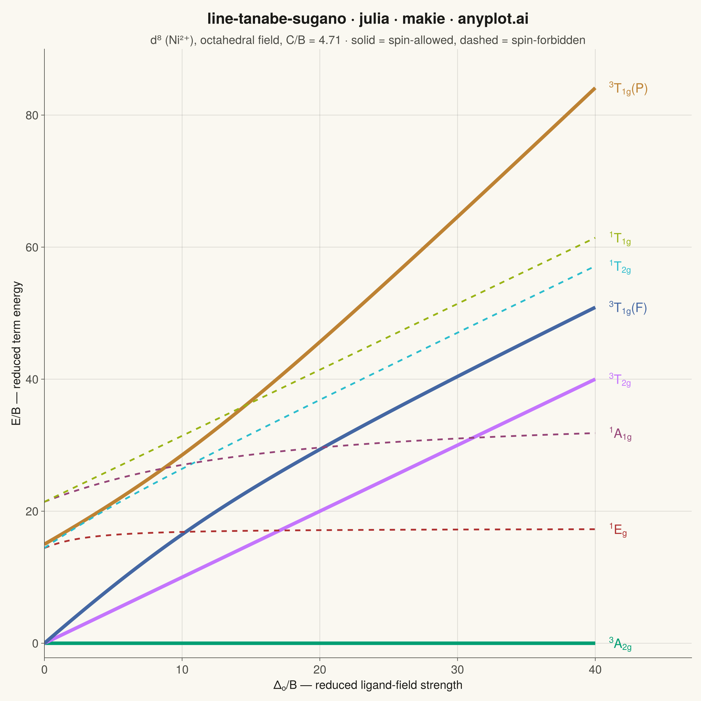
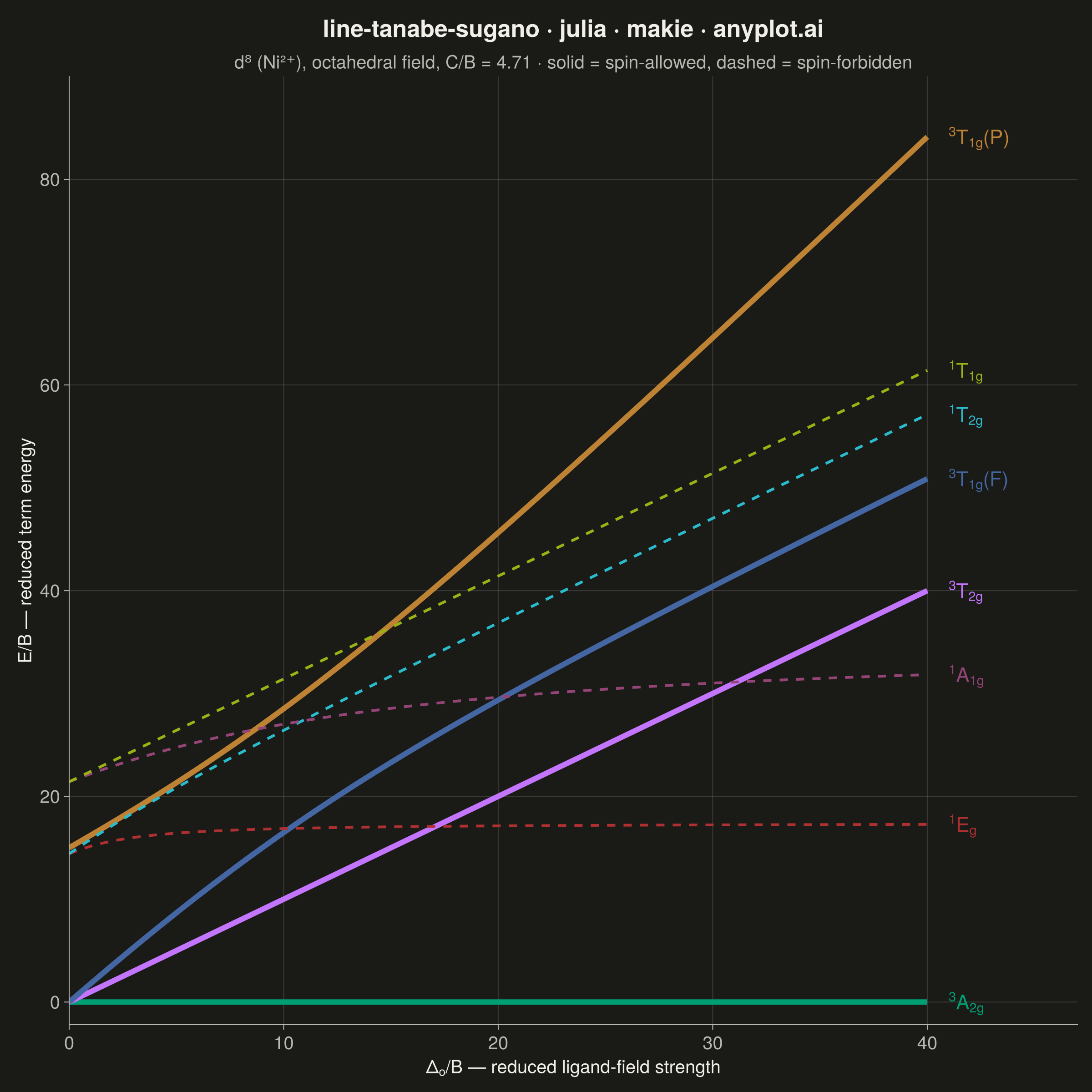
A Tanabe-Sugano diagram plots the energies of the electronic term states of a transition-metal ion in an octahedral ligand field as continuous functions of the field strength. The x-axis is the reduced ligand-field strength Δ_o/B (octahedral splitting divided by the Racah parameter B) and the y-axis is the reduced term energy E/B measured from the ground term, which therefore runs along the x-axis itself as a horizontal line at E/B = 0. Each term — labeled with its full symbol including spin multiplicity and Mulliken label — is one curve, and for d⁴–d⁷ a vertical line marks the high-spin/low-spin crossover where the ground term changes and every curve kinks. Chemists read the chart in reverse: matching ratios of observed UV-Vis band energies against the curves yields both Δ_o and B for a real complex.
# anyplot.ai
# line-tanabe-sugano: Tanabe-Sugano Diagram for Crystal Field Theory
# Library: makie 0.21.9 | Julia 1.11.9
# Quality: 89/100 | Created: 2026-10-01

using CairoMakie
using Colors
using LinearAlgebra

# Theme tokens — see prompts/default-style-guide.md "Theme-adaptive Chrome"
const THEME    = get(ENV, "ANYPLOT_THEME", "light")
const PAGE_BG  = THEME == "light" ? colorant"#FAF8F1" : colorant"#1A1A17"
const INK      = THEME == "light" ? colorant"#1A1A17" : colorant"#F0EFE8"
const INK_SOFT = THEME == "light" ? colorant"#4A4A44" : colorant"#B8B7B0"

# Imprint palette — positions 1-8 in canonical order, one per term curve
const IMPRINT_PALETTE = [
    colorant"#009E73", colorant"#C475FD", colorant"#4467A3", colorant"#BD8233",
    colorant"#AE3030", colorant"#2ABCCD", colorant"#954477", colorant"#99B314",
]

# Data — d⁸ (Ni²⁺) octahedral terms, all energies in units of the Racah B
c_over_b = 4.71
delta_over_b = range(0, 40, length = 320)
dq = delta_over_b ./ 10

# Free-ion term energies relative to ³F, from the Racah parameters B and C
e_3p = 15.0
e_1d = 5.0 + 2 * c_over_b
e_1g = 12.0 + 2 * c_over_b
e_1s = 22.0 + 7 * c_over_b

# Each symmetry block is a Tanabe-Sugano matrix: free-ion energies on the
# diagonal plus Dq times the ligand-field coupling, diagonalized per Δ_o/B
mix_eg = 40 * sqrt(3) / 7
mix_t2g = 20 * sqrt(3) / 7
mix_a1g = 4 * sqrt(6)

free_t1g = [0.0 0.0; 0.0 e_3p]
field_t1g = [6.0 4.0; 4.0 0.0]
free_singlet = [e_1d 0.0; 0.0 e_1g]
field_eg = [-24/7 mix_eg; mix_eg -4/7]
field_t2g = [16/7 mix_t2g; mix_t2g 26/7]
free_a1g = [e_1g 0.0; 0.0 e_1s]
field_a1g = [-4.0 mix_a1g; mix_a1g 0.0]

# The ³A₂g ground term lies at -12Dq, so +12q puts every curve on the E/B scale
t1g = [eigvals(Symmetric(free_t1g .+ q .* field_t1g)) .+ 12q for q in dq]
eg = [eigvals(Symmetric(free_singlet .+ q .* field_eg)) .+ 12q for q in dq]
t2g = [eigvals(Symmetric(free_singlet .+ q .* field_t2g)) .+ 12q for q in dq]
a1g = [eigvals(Symmetric(free_a1g .+ q .* field_a1g)) .+ 12q for q in dq]

# Term symbol, curve, palette position, and whether the spin is ground-term spin
terms = [
    (rich(superscript("3"), "A", subscript("2g")), zeros(length(dq)), 1, true),
    (rich(superscript("3"), "T", subscript("2g")), collect(delta_over_b), 2, true),
    (rich(superscript("3"), "T", subscript("1g"), "(F)"), first.(t1g), 3, true),
    (rich(superscript("3"), "T", subscript("1g"), "(P)"), last.(t1g), 4, true),
    (rich(superscript("1"), "E", subscript("g")), first.(eg), 5, false),
    (rich(superscript("1"), "T", subscript("2g")), first.(t2g), 6, false),
    (rich(superscript("1"), "A", subscript("1g")), first.(a1g), 7, false),
    (rich(superscript("1"), "T", subscript("1g")), e_1g .+ 10 .* dq, 8, false),
]

# Plot
fig = Figure(size = (1200, 1200), fontsize = 20, backgroundcolor = PAGE_BG)

ax = Axis(
    fig[1, 1];
    title = "line-tanabe-sugano · julia · makie · anyplot.ai",
    titlesize = 26,
    titlecolor = INK,
    subtitle = "d⁸ (Ni²⁺), octahedral field, C/B = 4.71 · solid = spin-allowed, dashed = spin-forbidden",
    subtitlesize = 20,
    subtitlecolor = INK_SOFT,
    subtitlegap = 10,
    xlabel = rich("Δ", subscript("o"), "/B — reduced ligand-field strength"),
    ylabel = "E/B — reduced term energy",
    xlabelsize = 20,
    ylabelsize = 20,
    xlabelcolor = INK,
    ylabelcolor = INK,
    xticklabelsize = 20,
    yticklabelsize = 20,
    xticklabelcolor = INK_SOFT,
    yticklabelcolor = INK_SOFT,
    xtickcolor = INK_SOFT,
    ytickcolor = INK_SOFT,
    xticks = 0:10:40,
    yticks = 0:20:80,
    backgroundcolor = PAGE_BG,
    topspinevisible = false,
    rightspinevisible = false,
    leftspinecolor = INK_SOFT,
    bottomspinecolor = INK_SOFT,
    xgridcolor = RGBAf(INK.r, INK.g, INK.b, 0.15),
    ygridcolor = RGBAf(INK.r, INK.g, INK.b, 0.15),
    xminorgridvisible = false,
    yminorgridvisible = false,
    limits = (0, 47, -2.2, 90),
)

for (symbol, energy, position, spin_allowed) in terms
    lines!(
        ax, delta_over_b, energy;
        color = IMPRINT_PALETTE[position],
        linewidth = spin_allowed ? 6 : 3,
        linestyle = spin_allowed ? :solid : :dash,
    )
    text!(
        ax, 41.0, energy[end];
        text = symbol,
        color = IMPRINT_PALETTE[position],
        fontsize = 22,
        align = (:left, :center),
    )
end

# Save
save("plot-$(THEME).png", fig; px_per_unit = 2)
Runnable source as JSON, for any HTTP client: https://api.anyplot.ai/specs/line-tanabe-sugano/makie/code. Any spec id and library id listed in llms-full.txt fit the same URL shape; every URL below is complete and callable.
{
  "spec_id": "line-tanabe-sugano",
  "language": "julia",
  "library": "makie",
  "page": "https://anyplot.ai/line-tanabe-sugano/julia/makie",
  "hub": "https://anyplot.ai/line-tanabe-sugano",
  "code_json": "https://api.anyplot.ai/specs/line-tanabe-sugano/makie/code",
  "spec_json": "https://api.anyplot.ai/specs/line-tanabe-sugano",
  "render_light_png": "https://storage.googleapis.com/anyplot-images/plots/line-tanabe-sugano/julia/makie/plot-light.png",
  "render_dark_png": "https://storage.googleapis.com/anyplot-images/plots/line-tanabe-sugano/julia/makie/plot-dark.png",
  "quality_score": 89.0,
  "license": "MIT",
  "guide": "https://anyplot.ai/llms.txt"
}
Part of Tanabe-Sugano Diagram for Crystal Field Theory on anyplot.ai.